A practical guide to making better decisions with data — from statistical foundations to experimentation culture
• Every experiment follows the same statistical chain: observe, summarise, quantify uncertainty, compare, decide.
• You don't need a stats degree — but you do need to understand what each step tells you and why it matters.
• This post builds the full pipeline visually, from raw data to hypothesis testing.
The Journey at a Glance
Before we dive in, here’s the full path we’ll walk. Each step builds on the last.
%3btext-align:center%3b%7d%23mermaid-0 .edgeLabel p%7bbackground-color:rgba(232%2c232%2c232%2c 0.8)%3b%7d%23mermaid-0 .edgeLabel rect%7bopacity:0.5%3bbackground-color:rgba(232%2c232%2c232%2c 0.8)%3bfill:rgba(232%2c232%2c232%2c 0.8)%3b%7d%23mermaid-0 .labelBkg%7bbackground-color:rgba(232%2c 232%2c 232%2c 0.5)%3b%7d%23mermaid-0 .cluster rect%7bfill:%23ffffde%3bstroke:%23aaaa33%3bstroke-width:1px%3b%7d%23mermaid-0 .cluster text%7bfill:%23333%3b%7d%23mermaid-0 .cluster span%7bcolor:%23333%3b%7d%23mermaid-0 div.mermaidTooltip%7bposition:absolute%3btext-align:center%3bmax-width:200px%3bpadding:2px%3bfont-family:arial%2csans-serif%3bfont-size:12px%3bbackground:hsl(80%2c 100%25%2c 96.2745098039%25)%3bborder:1px solid %23aaaa33%3bborder-radius:2px%3bpointer-events:none%3bz-index:100%3b%7d%23mermaid-0 .flowchartTitleText%7btext-anchor:middle%3bfont-size:18px%3bfill:%23333%3b%7d%23mermaid-0 rect.text%7bfill:none%3bstroke-width:0%3b%7d%23mermaid-0 .icon-shape%2c%23mermaid-0 .image-shape%7bbackground-color:rgba(232%2c232%2c232%2c 0.8)%3btext-align:center%3b%7d%23mermaid-0 .icon-shape p%2c%23mermaid-0 .image-shape p%7bbackground-color:rgba(232%2c232%2c232%2c 0.8)%3bpadding:2px%3b%7d%23mermaid-0 .icon-shape rect%2c%23mermaid-0 .image-shape rect%7bopacity:0.5%3bbackground-color:rgba(232%2c232%2c232%2c 0.8)%3bfill:rgba(232%2c232%2c232%2c 0.8)%3b%7d%23mermaid-0 .label-icon%7bdisplay:inline-block%3bheight:1em%3boverflow:visible%3bvertical-align:-0.125em%3b%7d%23mermaid-0 .node .label-icon path%7bfill:currentColor%3bstroke:revert%3bstroke-width:revert%3b%7d%23mermaid-0 :root%7b--mermaid-font-family:arial%2csans-serif%3b%7d%3c/style%3e%3cg%3e%3cmarker id='mermaid-0_flowchart-v2-pointEnd' class='marker flowchart-v2' viewBox='0 0 10 10' refX='5' refY='5' markerUnits='userSpaceOnUse' markerWidth='8' markerHeight='8' orient='auto'%3e%3cpath d='M 0 0 L 10 5 L 0 10 z' class='arrowMarkerPath' style='stroke-width: 1%3b stroke-dasharray: 1%2c 0%3b'/%3e%3c/marker%3e%3cmarker id='mermaid-0_flowchart-v2-pointStart' class='marker flowchart-v2' viewBox='0 0 10 10' refX='4.5' refY='5' markerUnits='userSpaceOnUse' markerWidth='8' markerHeight='8' orient='auto'%3e%3cpath d='M 0 5 L 10 10 L 10 0 z' class='arrowMarkerPath' style='stroke-width: 1%3b stroke-dasharray: 1%2c 0%3b'/%3e%3c/marker%3e%3cmarker id='mermaid-0_flowchart-v2-circleEnd' class='marker flowchart-v2' viewBox='0 0 10 10' refX='11' refY='5' markerUnits='userSpaceOnUse' markerWidth='11' markerHeight='11' orient='auto'%3e%3ccircle cx='5' cy='5' r='5' class='arrowMarkerPath' style='stroke-width: 1%3b stroke-dasharray: 1%2c 0%3b'/%3e%3c/marker%3e%3cmarker id='mermaid-0_flowchart-v2-circleStart' class='marker flowchart-v2' viewBox='0 0 10 10' refX='-1' refY='5' markerUnits='userSpaceOnUse' markerWidth='11' markerHeight='11' orient='auto'%3e%3ccircle cx='5' cy='5' r='5' class='arrowMarkerPath' style='stroke-width: 1%3b stroke-dasharray: 1%2c 0%3b'/%3e%3c/marker%3e%3cmarker id='mermaid-0_flowchart-v2-crossEnd' class='marker cross flowchart-v2' viewBox='0 0 11 11' refX='12' refY='5.2' markerUnits='userSpaceOnUse' markerWidth='11' markerHeight='11' orient='auto'%3e%3cpath d='M 1%2c1 l 9%2c9 M 10%2c1 l -9%2c9' class='arrowMarkerPath' style='stroke-width: 2%3b stroke-dasharray: 1%2c 0%3b'/%3e%3c/marker%3e%3cmarker id='mermaid-0_flowchart-v2-crossStart' class='marker cross flowchart-v2' viewBox='0 0 11 11' refX='-1' refY='5.2' markerUnits='userSpaceOnUse' markerWidth='11' markerHeight='11' orient='auto'%3e%3cpath d='M 1%2c1 l 9%2c9 M 10%2c1 l -9%2c9' class='arrowMarkerPath' style='stroke-width: 2%3b stroke-dasharray: 1%2c 0%3b'/%3e%3c/marker%3e%3cg class='root'%3e%3cg class='clusters'/%3e%3cg class='edgePaths'%3e%3cpath d='M138.25%2c35L142.417%2c35C146.583%2c35%2c154.917%2c35%2c162.583%2c35C170.25%2c35%2c177.25%2c35%2c180.75%2c35L184.25%2c35' id='L_A_B_0' class='edge-thickness-normal edge-pattern-solid edge-thickness-normal edge-pattern-solid flowchart-link' style='%3b' data-edge='true' data-et='edge' data-id='L_A_B_0' data-points='W3sieCI6MTM4LjI1LCJ5IjozNX0seyJ4IjoxNjMuMjUsInkiOjM1fSx7IngiOjE4OC4yNSwieSI6MzV9XQ==' marker-end='url(%23mermaid-0_flowchart-v2-pointEnd)'/%3e%3cpath d='M288.281%2c35L292.448%2c35C296.615%2c35%2c304.948%2c35%2c312.615%2c35C320.281%2c35%2c327.281%2c35%2c330.781%2c35L334.281%2c35' id='L_B_C_0' class='edge-thickness-normal edge-pattern-solid edge-thickness-normal edge-pattern-solid flowchart-link' style='%3b' data-edge='true' data-et='edge' data-id='L_B_C_0' data-points='W3sieCI6Mjg4LjI4MTI1LCJ5IjozNX0seyJ4IjozMTMuMjgxMjUsInkiOjM1fSx7IngiOjMzOC4yODEyNSwieSI6MzV9XQ==' marker-end='url(%23mermaid-0_flowchart-v2-pointEnd)'/%3e%3cpath d='M455.203%2c35L459.37%2c35C463.536%2c35%2c471.87%2c35%2c479.536%2c35C487.203%2c35%2c494.203%2c35%2c497.703%2c35L501.203%2c35' id='L_C_D_0' class='edge-thickness-normal edge-pattern-solid edge-thickness-normal edge-pattern-solid flowchart-link' style='%3b' data-edge='true' data-et='edge' data-id='L_C_D_0' data-points='W3sieCI6NDU1LjIwMzEyNSwieSI6MzV9LHsieCI6NDgwLjIwMzEyNSwieSI6MzV9LHsieCI6NTA1LjIwMzEyNSwieSI6MzV9XQ==' marker-end='url(%23mermaid-0_flowchart-v2-pointEnd)'/%3e%3cpath d='M629.219%2c35L633.385%2c35C637.552%2c35%2c645.885%2c35%2c653.552%2c35C661.219%2c35%2c668.219%2c35%2c671.719%2c35L675.219%2c35' id='L_D_E_0' class='edge-thickness-normal edge-pattern-solid edge-thickness-normal edge-pattern-solid flowchart-link' style='%3b' data-edge='true' data-et='edge' data-id='L_D_E_0' data-points='W3sieCI6NjI5LjIxODc1LCJ5IjozNX0seyJ4Ijo2NTQuMjE4NzUsInkiOjM1fSx7IngiOjY3OS4yMTg3NSwieSI6MzV9XQ==' marker-end='url(%23mermaid-0_flowchart-v2-pointEnd)'/%3e%3cpath d='M874.375%2c35L878.542%2c35C882.708%2c35%2c891.042%2c35%2c898.708%2c35C906.375%2c35%2c913.375%2c35%2c916.875%2c35L920.375%2c35' id='L_E_F_0' class='edge-thickness-normal edge-pattern-solid edge-thickness-normal edge-pattern-solid flowchart-link' style='%3b' data-edge='true' data-et='edge' data-id='L_E_F_0' data-points='W3sieCI6ODc0LjM3NSwieSI6MzV9LHsieCI6ODk5LjM3NSwieSI6MzV9LHsieCI6OTI0LjM3NSwieSI6MzV9XQ==' marker-end='url(%23mermaid-0_flowchart-v2-pointEnd)'/%3e%3cpath d='M1036.828%2c35L1040.995%2c35C1045.161%2c35%2c1053.495%2c35%2c1061.161%2c35C1068.828%2c35%2c1075.828%2c35%2c1079.328%2c35L1082.828%2c35' id='L_F_G_0' class='edge-thickness-normal edge-pattern-solid edge-thickness-normal edge-pattern-solid flowchart-link' style='%3b' data-edge='true' data-et='edge' data-id='L_F_G_0' data-points='W3sieCI6MTAzNi44MjgxMjUsInkiOjM1fSx7IngiOjEwNjEuODI4MTI1LCJ5IjozNX0seyJ4IjoxMDg2LjgyODEyNSwieSI6MzV9XQ==' marker-end='url(%23mermaid-0_flowchart-v2-pointEnd)'/%3e%3c/g%3e%3cg class='edgeLabels'%3e%3cg class='edgeLabel'%3e%3cg class='label' data-id='L_A_B_0' transform='translate(0%2c 0)'%3e%3cforeignObject width='0' height='0'%3e%3cdiv xmlns='http://www.w3.org/1999/xhtml' class='labelBkg' style='display: table-cell%3b white-space: nowrap%3b line-height: 1.5%3b max-width: 200px%3b text-align: center%3b'%3e%3cspan class='edgeLabel'%3e%3c/span%3e%3c/div%3e%3c/foreignObject%3e%3c/g%3e%3c/g%3e%3cg class='edgeLabel'%3e%3cg class='label' data-id='L_B_C_0' transform='translate(0%2c 0)'%3e%3cforeignObject width='0' height='0'%3e%3cdiv xmlns='http://www.w3.org/1999/xhtml' class='labelBkg' style='display: table-cell%3b white-space: nowrap%3b line-height: 1.5%3b max-width: 200px%3b text-align: center%3b'%3e%3cspan class='edgeLabel'%3e%3c/span%3e%3c/div%3e%3c/foreignObject%3e%3c/g%3e%3c/g%3e%3cg class='edgeLabel'%3e%3cg class='label' data-id='L_C_D_0' transform='translate(0%2c 0)'%3e%3cforeignObject width='0' height='0'%3e%3cdiv xmlns='http://www.w3.org/1999/xhtml' class='labelBkg' style='display: table-cell%3b white-space: nowrap%3b line-height: 1.5%3b max-width: 200px%3b text-align: center%3b'%3e%3cspan class='edgeLabel'%3e%3c/span%3e%3c/div%3e%3c/foreignObject%3e%3c/g%3e%3c/g%3e%3cg class='edgeLabel'%3e%3cg class='label' data-id='L_D_E_0' transform='translate(0%2c 0)'%3e%3cforeignObject width='0' height='0'%3e%3cdiv xmlns='http://www.w3.org/1999/xhtml' class='labelBkg' style='display: table-cell%3b white-space: nowrap%3b line-height: 1.5%3b max-width: 200px%3b text-align: center%3b'%3e%3cspan class='edgeLabel'%3e%3c/span%3e%3c/div%3e%3c/foreignObject%3e%3c/g%3e%3c/g%3e%3cg class='edgeLabel'%3e%3cg class='label' data-id='L_E_F_0' transform='translate(0%2c 0)'%3e%3cforeignObject width='0' height='0'%3e%3cdiv xmlns='http://www.w3.org/1999/xhtml' class='labelBkg' style='display: table-cell%3b white-space: nowrap%3b line-height: 1.5%3b max-width: 200px%3b text-align: center%3b'%3e%3cspan class='edgeLabel'%3e%3c/span%3e%3c/div%3e%3c/foreignObject%3e%3c/g%3e%3c/g%3e%3cg class='edgeLabel'%3e%3cg class='label' data-id='L_F_G_0' transform='translate(0%2c 0)'%3e%3cforeignObject width='0' height='0'%3e%3cdiv xmlns='http://www.w3.org/1999/xhtml' class='labelBkg' style='display: table-cell%3b white-space: nowrap%3b line-height: 1.5%3b max-width: 200px%3b text-align: center%3b'%3e%3cspan class='edgeLabel'%3e%3c/span%3e%3c/div%3e%3c/foreignObject%3e%3c/g%3e%3c/g%3e%3c/g%3e%3cg class='nodes'%3e%3cg class='node default' id='flowchart-A-0' transform='translate(73.125%2c 35)'%3e%3crect class='basic label-container' style='fill:%234a9eff !important%3bstroke:none !important' x='-65.125' y='-27' width='130.25' height='54'/%3e%3cg class='label' style='color:white !important' transform='translate(-35.125%2c -12)'%3e%3crect/%3e%3cforeignObject width='70.25' height='24'%3e%3cdiv style='color: rgb(255%2c 255%2c 255) !important%3b display: table-cell%3b white-space: nowrap%3b line-height: 1.5%3b max-width: 200px%3b text-align: center%3b' xmlns='http://www.w3.org/1999/xhtml'%3e%3cspan style='color:white !important' class='nodeLabel'%3e%3cp%3eRaw Data%3c/p%3e%3c/span%3e%3c/div%3e%3c/foreignObject%3e%3c/g%3e%3c/g%3e%3cg class='node default' id='flowchart-B-1' transform='translate(238.265625%2c 35)'%3e%3crect class='basic label-container' style='fill:%2322c55e !important%3bstroke:none !important' x='-50.015625' y='-27' width='100.03125' height='54'/%3e%3cg class='label' style='color:white !important' transform='translate(-20.015625%2c -12)'%3e%3crect/%3e%3cforeignObject width='40.03125' height='24'%3e%3cdiv style='color: rgb(255%2c 255%2c 255) !important%3b display: table-cell%3b white-space: nowrap%3b line-height: 1.5%3b max-width: 200px%3b text-align: center%3b' xmlns='http://www.w3.org/1999/xhtml'%3e%3cspan style='color:white !important' class='nodeLabel'%3e%3cp%3eMean%3c/p%3e%3c/span%3e%3c/div%3e%3c/foreignObject%3e%3c/g%3e%3c/g%3e%3cg class='node default' id='flowchart-C-3' transform='translate(396.7421875%2c 35)'%3e%3crect class='basic label-container' style='fill:%23f97316 !important%3bstroke:none !important' x='-58.4609375' y='-27' width='116.921875' height='54'/%3e%3cg class='label' style='color:white !important' transform='translate(-28.4609375%2c -12)'%3e%3crect/%3e%3cforeignObject width='56.921875' height='24'%3e%3cdiv style='color: rgb(255%2c 255%2c 255) !important%3b display: table-cell%3b white-space: nowrap%3b line-height: 1.5%3b max-width: 200px%3b text-align: center%3b' xmlns='http://www.w3.org/1999/xhtml'%3e%3cspan style='color:white !important' class='nodeLabel'%3e%3cp%3eStd Dev%3c/p%3e%3c/span%3e%3c/div%3e%3c/foreignObject%3e%3c/g%3e%3c/g%3e%3cg class='node default' id='flowchart-D-5' transform='translate(567.2109375%2c 35)'%3e%3crect class='basic label-container' style='fill:%23eab308 !important%3bstroke:none !important' x='-62.0078125' y='-27' width='124.015625' height='54'/%3e%3cg class='label' style='color:white !important' transform='translate(-32.0078125%2c -12)'%3e%3crect/%3e%3cforeignObject width='64.015625' height='24'%3e%3cdiv style='color: rgb(255%2c 255%2c 255) !important%3b display: table-cell%3b white-space: nowrap%3b line-height: 1.5%3b max-width: 200px%3b text-align: center%3b' xmlns='http://www.w3.org/1999/xhtml'%3e%3cspan style='color:white !important' class='nodeLabel'%3e%3cp%3eStd Error%3c/p%3e%3c/span%3e%3c/div%3e%3c/foreignObject%3e%3c/g%3e%3c/g%3e%3cg class='node default' id='flowchart-E-7' transform='translate(776.796875%2c 35)'%3e%3crect class='basic label-container' style='fill:%23ef4444 !important%3bstroke:none !important' x='-97.578125' y='-27' width='195.15625' height='54'/%3e%3cg class='label' style='color:white !important' transform='translate(-67.578125%2c -12)'%3e%3crect/%3e%3cforeignObject width='135.15625' height='24'%3e%3cdiv style='color: rgb(255%2c 255%2c 255) !important%3b display: table-cell%3b white-space: nowrap%3b line-height: 1.5%3b max-width: 200px%3b text-align: center%3b' xmlns='http://www.w3.org/1999/xhtml'%3e%3cspan style='color:white !important' class='nodeLabel'%3e%3cp%3eCompare%5cn(A vs B)%3c/p%3e%3c/span%3e%3c/div%3e%3c/foreignObject%3e%3c/g%3e%3c/g%3e%3cg class='node default' id='flowchart-F-9' transform='translate(980.6015625%2c 35)'%3e%3crect class='basic label-container' style='fill:%23a855f7 !important%3bstroke:none !important' x='-56.2265625' y='-27' width='112.453125' height='54'/%3e%3cg class='label' style='color:white !important' transform='translate(-26.2265625%2c -12)'%3e%3crect/%3e%3cforeignObject width='52.453125' height='24'%3e%3cdiv style='color: rgb(255%2c 255%2c 255) !important%3b display: table-cell%3b white-space: nowrap%3b line-height: 1.5%3b max-width: 200px%3b text-align: center%3b' xmlns='http://www.w3.org/1999/xhtml'%3e%3cspan style='color:white !important' class='nodeLabel'%3e%3cp%3ez-score%3c/p%3e%3c/span%3e%3c/div%3e%3c/foreignObject%3e%3c/g%3e%3c/g%3e%3cg class='node default' id='flowchart-G-11' transform='translate(1147.5078125%2c 35)'%3e%3crect class='basic label-container' style='fill:%236366f1 !important%3bstroke:none !important' x='-60.6796875' y='-27' width='121.359375' height='54'/%3e%3cg class='label' style='color:white !important' transform='translate(-30.6796875%2c -12)'%3e%3crect/%3e%3cforeignObject width='61.359375' height='24'%3e%3cdiv style='color: rgb(255%2c 255%2c 255) !important%3b display: table-cell%3b white-space: nowrap%3b line-height: 1.5%3b max-width: 200px%3b text-align: center%3b' xmlns='http://www.w3.org/1999/xhtml'%3e%3cspan style='color:white !important' class='nodeLabel'%3e%3cp%3eDecision%3c/p%3e%3c/span%3e%3c/div%3e%3c/foreignObject%3e%3c/g%3e%3c/g%3e%3c/g%3e%3c/g%3e%3c/g%3e%3c/svg%3e)
Each coloured block is a section below. By the end, you’ll understand how noisy observations become principled business decisions.
The Setup
Imagine you own a small coffee shop with two baristas — Anna and Ben.
Customers queue up. You start timing how long each one waits from order to drink in hand. Your question is simple:
Is one barista meaningfully faster than the other?
This is the same question behind every A/B test, every feature experiment, every pricing change. The domain differs; the statistical machinery is identical.
%3btext-align:center%3b%7d%23mermaid-1 .edgeLabel p%7bbackground-color:rgba(232%2c232%2c232%2c 0.8)%3b%7d%23mermaid-1 .edgeLabel rect%7bopacity:0.5%3bbackground-color:rgba(232%2c232%2c232%2c 0.8)%3bfill:rgba(232%2c232%2c232%2c 0.8)%3b%7d%23mermaid-1 .labelBkg%7bbackground-color:rgba(232%2c 232%2c 232%2c 0.5)%3b%7d%23mermaid-1 .cluster rect%7bfill:%23ffffde%3bstroke:%23aaaa33%3bstroke-width:1px%3b%7d%23mermaid-1 .cluster text%7bfill:%23333%3b%7d%23mermaid-1 .cluster span%7bcolor:%23333%3b%7d%23mermaid-1 div.mermaidTooltip%7bposition:absolute%3btext-align:center%3bmax-width:200px%3bpadding:2px%3bfont-family:arial%2csans-serif%3bfont-size:12px%3bbackground:hsl(80%2c 100%25%2c 96.2745098039%25)%3bborder:1px solid %23aaaa33%3bborder-radius:2px%3bpointer-events:none%3bz-index:100%3b%7d%23mermaid-1 .flowchartTitleText%7btext-anchor:middle%3bfont-size:18px%3bfill:%23333%3b%7d%23mermaid-1 rect.text%7bfill:none%3bstroke-width:0%3b%7d%23mermaid-1 .icon-shape%2c%23mermaid-1 .image-shape%7bbackground-color:rgba(232%2c232%2c232%2c 0.8)%3btext-align:center%3b%7d%23mermaid-1 .icon-shape p%2c%23mermaid-1 .image-shape p%7bbackground-color:rgba(232%2c232%2c232%2c 0.8)%3bpadding:2px%3b%7d%23mermaid-1 .icon-shape rect%2c%23mermaid-1 .image-shape rect%7bopacity:0.5%3bbackground-color:rgba(232%2c232%2c232%2c 0.8)%3bfill:rgba(232%2c232%2c232%2c 0.8)%3b%7d%23mermaid-1 .label-icon%7bdisplay:inline-block%3bheight:1em%3boverflow:visible%3bvertical-align:-0.125em%3b%7d%23mermaid-1 .node .label-icon path%7bfill:currentColor%3bstroke:revert%3bstroke-width:revert%3b%7d%23mermaid-1 :root%7b--mermaid-font-family:arial%2csans-serif%3b%7d%3c/style%3e%3cg%3e%3cmarker id='mermaid-1_flowchart-v2-pointEnd' class='marker flowchart-v2' viewBox='0 0 10 10' refX='5' refY='5' markerUnits='userSpaceOnUse' markerWidth='8' markerHeight='8' orient='auto'%3e%3cpath d='M 0 0 L 10 5 L 0 10 z' class='arrowMarkerPath' style='stroke-width: 1%3b stroke-dasharray: 1%2c 0%3b'/%3e%3c/marker%3e%3cmarker id='mermaid-1_flowchart-v2-pointStart' class='marker flowchart-v2' viewBox='0 0 10 10' refX='4.5' refY='5' markerUnits='userSpaceOnUse' markerWidth='8' markerHeight='8' orient='auto'%3e%3cpath d='M 0 5 L 10 10 L 10 0 z' class='arrowMarkerPath' style='stroke-width: 1%3b stroke-dasharray: 1%2c 0%3b'/%3e%3c/marker%3e%3cmarker id='mermaid-1_flowchart-v2-circleEnd' class='marker flowchart-v2' viewBox='0 0 10 10' refX='11' refY='5' markerUnits='userSpaceOnUse' markerWidth='11' markerHeight='11' orient='auto'%3e%3ccircle cx='5' cy='5' r='5' class='arrowMarkerPath' style='stroke-width: 1%3b stroke-dasharray: 1%2c 0%3b'/%3e%3c/marker%3e%3cmarker id='mermaid-1_flowchart-v2-circleStart' class='marker flowchart-v2' viewBox='0 0 10 10' refX='-1' refY='5' markerUnits='userSpaceOnUse' markerWidth='11' markerHeight='11' orient='auto'%3e%3ccircle cx='5' cy='5' r='5' class='arrowMarkerPath' style='stroke-width: 1%3b stroke-dasharray: 1%2c 0%3b'/%3e%3c/marker%3e%3cmarker id='mermaid-1_flowchart-v2-crossEnd' class='marker cross flowchart-v2' viewBox='0 0 11 11' refX='12' refY='5.2' markerUnits='userSpaceOnUse' markerWidth='11' markerHeight='11' orient='auto'%3e%3cpath d='M 1%2c1 l 9%2c9 M 10%2c1 l -9%2c9' class='arrowMarkerPath' style='stroke-width: 2%3b stroke-dasharray: 1%2c 0%3b'/%3e%3c/marker%3e%3cmarker id='mermaid-1_flowchart-v2-crossStart' class='marker cross flowchart-v2' viewBox='0 0 11 11' refX='-1' refY='5.2' markerUnits='userSpaceOnUse' markerWidth='11' markerHeight='11' orient='auto'%3e%3cpath d='M 1%2c1 l 9%2c9 M 10%2c1 l -9%2c9' class='arrowMarkerPath' style='stroke-width: 2%3b stroke-dasharray: 1%2c 0%3b'/%3e%3c/marker%3e%3cg class='root'%3e%3cg class='clusters'/%3e%3cg class='edgePaths'%3e%3cpath d='M819.688%2c147L830.228%2c147C840.768%2c147%2c861.849%2c147%2c882.263%2c147C902.677%2c147%2c922.424%2c147%2c932.298%2c147L942.172%2c147' id='L_Q_STATS_0' class='edge-thickness-normal edge-pattern-solid edge-thickness-normal edge-pattern-solid flowchart-link' style='%3b' data-edge='true' data-et='edge' data-id='L_Q_STATS_0' data-points='W3sieCI6ODE5LjY4NzUsInkiOjE0N30seyJ4Ijo4ODIuOTI5Njg3NSwieSI6MTQ3fSx7IngiOjk0Ni4xNzE4NzUsInkiOjE0N31d' marker-end='url(%23mermaid-1_flowchart-v2-pointEnd)'/%3e%3cpath d='M491.688%2c147L495.854%2c147C500.021%2c147%2c508.354%2c147%2c516.021%2c147C523.688%2c147%2c530.688%2c147%2c534.188%2c147L537.688%2c147' id='L_shop_Q_0' class='edge-thickness-normal edge-pattern-solid edge-thickness-normal edge-pattern-solid flowchart-link' style='%3b' data-edge='true' data-et='edge' data-id='L_shop_Q_0' data-points='W3sieCI6NDkxLjY4NzUsInkiOjE0N30seyJ4Ijo1MTYuNjg3NSwieSI6MTQ3fSx7IngiOjU0MS42ODc1LCJ5IjoxNDd9XQ==' marker-end='url(%23mermaid-1_flowchart-v2-pointEnd)'/%3e%3c/g%3e%3cg class='edgeLabels'%3e%3cg class='edgeLabel' transform='translate(882.9296875%2c 147)'%3e%3cg class='label' data-id='L_Q_STATS_0' transform='translate(-38.2421875%2c -12)'%3e%3cforeignObject width='76.484375' height='24'%3e%3cdiv xmlns='http://www.w3.org/1999/xhtml' class='labelBkg' style='display: table-cell%3b white-space: nowrap%3b line-height: 1.5%3b max-width: 200px%3b text-align: center%3b'%3e%3cspan class='edgeLabel'%3e%3cp%3eNeed stats%3c/p%3e%3c/span%3e%3c/div%3e%3c/foreignObject%3e%3c/g%3e%3c/g%3e%3cg class='edgeLabel'%3e%3cg class='label' data-id='L_shop_Q_0' transform='translate(0%2c 0)'%3e%3cforeignObject width='0' height='0'%3e%3cdiv xmlns='http://www.w3.org/1999/xhtml' class='labelBkg' style='display: table-cell%3b white-space: nowrap%3b line-height: 1.5%3b max-width: 200px%3b text-align: center%3b'%3e%3cspan class='edgeLabel'%3e%3c/span%3e%3c/div%3e%3c/foreignObject%3e%3c/g%3e%3c/g%3e%3c/g%3e%3cg class='nodes'%3e%3cg class='root' transform='translate(0%2c 10)'%3e%3cg class='clusters'%3e%3cg class='cluster' id='shop' data-look='classic'%3e%3crect style='fill:%231e293b !important%3bstroke:%23334155 !important' x='8' y='8' width='483.6875' height='258'/%3e%3cg class='cluster-label' transform='translate(205.5078125%2c 8)'%3e%3cforeignObject width='88.671875' height='24'%3e%3cdiv xmlns='http://www.w3.org/1999/xhtml' style='display: table-cell%3b white-space: nowrap%3b line-height: 1.5%3b max-width: 200px%3b text-align: center%3b'%3e%3cspan class='nodeLabel' style='color:%2394a3b8 !important'%3e%3cp%3eCoffee Shop%3c/p%3e%3c/span%3e%3c/div%3e%3c/foreignObject%3e%3c/g%3e%3c/g%3e%3c/g%3e%3cg class='edgePaths'%3e%3cpath d='M133.922%2c99.5L133.922%2c105.75C133.922%2c112%2c133.922%2c124.5%2c133.922%2c137C133.922%2c149.5%2c133.922%2c162%2c133.922%2c168.25L133.922%2c174.5' id='L_C1_C2_0' class='edge-thickness-invisible edge-pattern-solid' style='%3b' data-edge='true' data-et='edge' data-id='L_C1_C2_0' data-points='W3sieCI6MTMzLjkyMTg3NSwieSI6OTkuNX0seyJ4IjoxMzMuOTIxODc1LCJ5IjoxMzd9LHsieCI6MTMzLjkyMTg3NSwieSI6MTc0LjV9XQ=='/%3e%3cpath d='M365.766%2c99.5L365.766%2c105.75C365.766%2c112%2c365.766%2c124.5%2c365.766%2c137C365.766%2c149.5%2c365.766%2c162%2c365.766%2c168.25L365.766%2c174.5' id='L_C3_C4_0' class='edge-thickness-invisible edge-pattern-solid' style='%3b' data-edge='true' data-et='edge' data-id='L_C3_C4_0' data-points='W3sieCI6MzY1Ljc2NTYyNSwieSI6OTkuNX0seyJ4IjozNjUuNzY1NjI1LCJ5IjoxMzd9LHsieCI6MzY1Ljc2NTYyNSwieSI6MTc0LjV9XQ=='/%3e%3c/g%3e%3cg class='edgeLabels'%3e%3cg class='edgeLabel'%3e%3cg class='label' data-id='L_C1_C2_0' transform='translate(0%2c 0)'%3e%3cforeignObject width='0' height='0'%3e%3cdiv xmlns='http://www.w3.org/1999/xhtml' class='labelBkg' style='display: table-cell%3b white-space: nowrap%3b line-height: 1.5%3b max-width: 200px%3b text-align: center%3b'%3e%3cspan class='edgeLabel'%3e%3c/span%3e%3c/div%3e%3c/foreignObject%3e%3c/g%3e%3c/g%3e%3cg class='edgeLabel'%3e%3cg class='label' data-id='L_C3_C4_0' transform='translate(0%2c 0)'%3e%3cforeignObject width='0' height='0'%3e%3cdiv xmlns='http://www.w3.org/1999/xhtml' class='labelBkg' style='display: table-cell%3b white-space: nowrap%3b line-height: 1.5%3b max-width: 200px%3b text-align: center%3b'%3e%3cspan class='edgeLabel'%3e%3c/span%3e%3c/div%3e%3c/foreignObject%3e%3c/g%3e%3c/g%3e%3c/g%3e%3cg class='nodes'%3e%3cg class='node default' id='flowchart-C1-0' transform='translate(133.921875%2c 72.5)'%3e%3crect class='basic label-container' style='' x='-90.921875' y='-27' width='181.84375' height='54'/%3e%3cg class='label' style='' transform='translate(-60.921875%2c -12)'%3e%3crect/%3e%3cforeignObject width='121.84375' height='24'%3e%3cdiv xmlns='http://www.w3.org/1999/xhtml' style='display: table-cell%3b white-space: nowrap%3b line-height: 1.5%3b max-width: 200px%3b text-align: center%3b'%3e%3cspan class='nodeLabel'%3e%3cp%3eCustomer 1%5cn18s%3c/p%3e%3c/span%3e%3c/div%3e%3c/foreignObject%3e%3c/g%3e%3c/g%3e%3cg class='node default' id='flowchart-C2-1' transform='translate(133.921875%2c 201.5)'%3e%3crect class='basic label-container' style='' x='-90.921875' y='-27' width='181.84375' height='54'/%3e%3cg class='label' style='' transform='translate(-60.921875%2c -12)'%3e%3crect/%3e%3cforeignObject width='121.84375' height='24'%3e%3cdiv xmlns='http://www.w3.org/1999/xhtml' style='display: table-cell%3b white-space: nowrap%3b line-height: 1.5%3b max-width: 200px%3b text-align: center%3b'%3e%3cspan class='nodeLabel'%3e%3cp%3eCustomer 2%5cn42s%3c/p%3e%3c/span%3e%3c/div%3e%3c/foreignObject%3e%3c/g%3e%3c/g%3e%3cg class='node default' id='flowchart-C3-2' transform='translate(365.765625%2c 72.5)'%3e%3crect class='basic label-container' style='' x='-90.921875' y='-27' width='181.84375' height='54'/%3e%3cg class='label' style='' transform='translate(-60.921875%2c -12)'%3e%3crect/%3e%3cforeignObject width='121.84375' height='24'%3e%3cdiv xmlns='http://www.w3.org/1999/xhtml' style='display: table-cell%3b white-space: nowrap%3b line-height: 1.5%3b max-width: 200px%3b text-align: center%3b'%3e%3cspan class='nodeLabel'%3e%3cp%3eCustomer 3%5cn65s%3c/p%3e%3c/span%3e%3c/div%3e%3c/foreignObject%3e%3c/g%3e%3c/g%3e%3cg class='node default' id='flowchart-C4-3' transform='translate(365.765625%2c 201.5)'%3e%3crect class='basic label-container' style='' x='-90.921875' y='-27' width='181.84375' height='54'/%3e%3cg class='label' style='' transform='translate(-60.921875%2c -12)'%3e%3crect/%3e%3cforeignObject width='121.84375' height='24'%3e%3cdiv xmlns='http://www.w3.org/1999/xhtml' style='display: table-cell%3b white-space: nowrap%3b line-height: 1.5%3b max-width: 200px%3b text-align: center%3b'%3e%3cspan class='nodeLabel'%3e%3cp%3eCustomer 4%5cn14s%3c/p%3e%3c/span%3e%3c/div%3e%3c/foreignObject%3e%3c/g%3e%3c/g%3e%3c/g%3e%3c/g%3e%3cg class='node default' id='flowchart-Q-5' transform='translate(680.6875%2c 147)'%3e%3cpolygon points='139%2c0 278%2c-139 139%2c-278 0%2c-139' class='label-container' transform='translate(-138.5%2c 139)' style='fill:%23f59e0b !important%3bstroke:none !important'/%3e%3cg class='label' style='color:black !important' transform='translate(-100%2c -24)'%3e%3crect/%3e%3cforeignObject width='200' height='48'%3e%3cdiv style='color: rgb(0%2c 0%2c 0) !important%3b display: table%3b white-space: break-spaces%3b line-height: 1.5%3b max-width: 200px%3b text-align: center%3b width: 200px%3b' xmlns='http://www.w3.org/1999/xhtml'%3e%3cspan style='color:black !important' class='nodeLabel'%3e%3cp%3eWho is faster%3f%5cnAnna or Ben%3f%3c/p%3e%3c/span%3e%3c/div%3e%3c/foreignObject%3e%3c/g%3e%3c/g%3e%3cg class='node default' id='flowchart-STATS-7' transform='translate(1045.546875%2c 147)'%3e%3crect class='basic label-container' style='fill:%234a9eff !important%3bstroke:none !important' x='-99.375' y='-27' width='198.75' height='54'/%3e%3cg class='label' style='color:white !important' transform='translate(-69.375%2c -12)'%3e%3crect/%3e%3cforeignObject width='138.75' height='24'%3e%3cdiv style='color: rgb(255%2c 255%2c 255) !important%3b display: table-cell%3b white-space: nowrap%3b line-height: 1.5%3b max-width: 200px%3b text-align: center%3b' xmlns='http://www.w3.org/1999/xhtml'%3e%3cspan style='color:white !important' class='nodeLabel'%3e%3cp%3eStatistical%5cnPipeline%3c/p%3e%3c/span%3e%3c/div%3e%3c/foreignObject%3e%3c/g%3e%3c/g%3e%3c/g%3e%3c/g%3e%3c/g%3e%3c/svg%3e)
Step 1: The Mean — What’s “Typical”?
After timing many customers, you compute each barista’s average:
| Barista | Mean Wait Time |
|---|---|
| Anna | 28 seconds |
| Ben | 31 seconds |
- Mean (Average)
-
The balancing point of all observations. If you placed every wait time as a weight on a number line, the mean is where the plank balances.
The mean compresses messy reality into a single representative number. It’s the value that minimises the sum of squared distances from every data point — the optimal single summary.
%3btext-align:center%3b%7d%23mermaid-2 .edgeLabel p%7bbackground-color:rgba(232%2c232%2c232%2c 0.8)%3b%7d%23mermaid-2 .edgeLabel rect%7bopacity:0.5%3bbackground-color:rgba(232%2c232%2c232%2c 0.8)%3bfill:rgba(232%2c232%2c232%2c 0.8)%3b%7d%23mermaid-2 .labelBkg%7bbackground-color:rgba(232%2c 232%2c 232%2c 0.5)%3b%7d%23mermaid-2 .cluster rect%7bfill:%23ffffde%3bstroke:%23aaaa33%3bstroke-width:1px%3b%7d%23mermaid-2 .cluster text%7bfill:%23333%3b%7d%23mermaid-2 .cluster span%7bcolor:%23333%3b%7d%23mermaid-2 div.mermaidTooltip%7bposition:absolute%3btext-align:center%3bmax-width:200px%3bpadding:2px%3bfont-family:arial%2csans-serif%3bfont-size:12px%3bbackground:hsl(80%2c 100%25%2c 96.2745098039%25)%3bborder:1px solid %23aaaa33%3bborder-radius:2px%3bpointer-events:none%3bz-index:100%3b%7d%23mermaid-2 .flowchartTitleText%7btext-anchor:middle%3bfont-size:18px%3bfill:%23333%3b%7d%23mermaid-2 rect.text%7bfill:none%3bstroke-width:0%3b%7d%23mermaid-2 .icon-shape%2c%23mermaid-2 .image-shape%7bbackground-color:rgba(232%2c232%2c232%2c 0.8)%3btext-align:center%3b%7d%23mermaid-2 .icon-shape p%2c%23mermaid-2 .image-shape p%7bbackground-color:rgba(232%2c232%2c232%2c 0.8)%3bpadding:2px%3b%7d%23mermaid-2 .icon-shape rect%2c%23mermaid-2 .image-shape rect%7bopacity:0.5%3bbackground-color:rgba(232%2c232%2c232%2c 0.8)%3bfill:rgba(232%2c232%2c232%2c 0.8)%3b%7d%23mermaid-2 .label-icon%7bdisplay:inline-block%3bheight:1em%3boverflow:visible%3bvertical-align:-0.125em%3b%7d%23mermaid-2 .node .label-icon path%7bfill:currentColor%3bstroke:revert%3bstroke-width:revert%3b%7d%23mermaid-2 :root%7b--mermaid-font-family:arial%2csans-serif%3b%7d%3c/style%3e%3cg%3e%3cmarker id='mermaid-2_flowchart-v2-pointEnd' class='marker flowchart-v2' viewBox='0 0 10 10' refX='5' refY='5' markerUnits='userSpaceOnUse' markerWidth='8' markerHeight='8' orient='auto'%3e%3cpath d='M 0 0 L 10 5 L 0 10 z' class='arrowMarkerPath' style='stroke-width: 1%3b stroke-dasharray: 1%2c 0%3b'/%3e%3c/marker%3e%3cmarker id='mermaid-2_flowchart-v2-pointStart' class='marker flowchart-v2' viewBox='0 0 10 10' refX='4.5' refY='5' markerUnits='userSpaceOnUse' markerWidth='8' markerHeight='8' orient='auto'%3e%3cpath d='M 0 5 L 10 10 L 10 0 z' class='arrowMarkerPath' style='stroke-width: 1%3b stroke-dasharray: 1%2c 0%3b'/%3e%3c/marker%3e%3cmarker id='mermaid-2_flowchart-v2-circleEnd' class='marker flowchart-v2' viewBox='0 0 10 10' refX='11' refY='5' markerUnits='userSpaceOnUse' markerWidth='11' markerHeight='11' orient='auto'%3e%3ccircle cx='5' cy='5' r='5' class='arrowMarkerPath' style='stroke-width: 1%3b stroke-dasharray: 1%2c 0%3b'/%3e%3c/marker%3e%3cmarker id='mermaid-2_flowchart-v2-circleStart' class='marker flowchart-v2' viewBox='0 0 10 10' refX='-1' refY='5' markerUnits='userSpaceOnUse' markerWidth='11' markerHeight='11' orient='auto'%3e%3ccircle cx='5' cy='5' r='5' class='arrowMarkerPath' style='stroke-width: 1%3b stroke-dasharray: 1%2c 0%3b'/%3e%3c/marker%3e%3cmarker id='mermaid-2_flowchart-v2-crossEnd' class='marker cross flowchart-v2' viewBox='0 0 11 11' refX='12' refY='5.2' markerUnits='userSpaceOnUse' markerWidth='11' markerHeight='11' orient='auto'%3e%3cpath d='M 1%2c1 l 9%2c9 M 10%2c1 l -9%2c9' class='arrowMarkerPath' style='stroke-width: 2%3b stroke-dasharray: 1%2c 0%3b'/%3e%3c/marker%3e%3cmarker id='mermaid-2_flowchart-v2-crossStart' class='marker cross flowchart-v2' viewBox='0 0 11 11' refX='-1' refY='5.2' markerUnits='userSpaceOnUse' markerWidth='11' markerHeight='11' orient='auto'%3e%3cpath d='M 1%2c1 l 9%2c9 M 10%2c1 l -9%2c9' class='arrowMarkerPath' style='stroke-width: 2%3b stroke-dasharray: 1%2c 0%3b'/%3e%3c/marker%3e%3cg class='root'%3e%3cg class='clusters'/%3e%3cg class='edgePaths'%3e%3cpath d='M357.859%2c266L362.026%2c266C366.193%2c266%2c374.526%2c266%2c391.716%2c308.03C408.905%2c350.06%2c434.951%2c434.119%2c447.974%2c476.149L460.997%2c518.179' id='L_MA_GAP_0' class='edge-thickness-normal edge-pattern-solid edge-thickness-normal edge-pattern-solid flowchart-link' style='%3b' data-edge='true' data-et='edge' data-id='L_MA_GAP_0' data-points='W3sieCI6MzU3Ljg1OTM3NSwieSI6MjY2fSx7IngiOjM4Mi44NTkzNzUsInkiOjI2Nn0seyJ4Ijo0NjIuMTgwOTI5NzcwMzE4LCJ5Ijo1MjJ9XQ==' marker-end='url(%23mermaid-2_flowchart-v2-pointEnd)'/%3e%3cpath d='M357.859%2c832L362.026%2c832C366.193%2c832%2c374.526%2c832%2c391.716%2c789.97C408.905%2c747.94%2c434.951%2c663.881%2c447.974%2c621.851L460.997%2c579.821' id='L_MB_GAP_0' class='edge-thickness-normal edge-pattern-solid edge-thickness-normal edge-pattern-solid flowchart-link' style='%3b' data-edge='true' data-et='edge' data-id='L_MB_GAP_0' data-points='W3sieCI6MzU3Ljg1OTM3NSwieSI6ODMyfSx7IngiOjM4Mi44NTkzNzUsInkiOjgzMn0seyJ4Ijo0NjIuMTgwOTI5NzcwMzE4LCJ5Ijo1NzZ9XQ==' marker-end='url(%23mermaid-2_flowchart-v2-pointEnd)'/%3e%3cpath d='M163.797%2c266L167.964%2c266C172.13%2c266%2c180.464%2c266%2c188.13%2c266C195.797%2c266%2c202.797%2c266%2c206.297%2c266L209.797%2c266' id='L_anna_MA_0' class='edge-thickness-normal edge-pattern-solid edge-thickness-normal edge-pattern-solid flowchart-link' style='%3b' data-edge='true' data-et='edge' data-id='L_anna_MA_0' data-points='W3sieCI6MTYzLjc5Njg3NSwieSI6MjY2fSx7IngiOjE4OC43OTY4NzUsInkiOjI2Nn0seyJ4IjoyMTMuNzk2ODc1LCJ5IjoyNjZ9XQ==' marker-end='url(%23mermaid-2_flowchart-v2-pointEnd)'/%3e%3cpath d='M163.797%2c832L167.964%2c832C172.13%2c832%2c180.464%2c832%2c188.13%2c832C195.797%2c832%2c202.797%2c832%2c206.297%2c832L209.797%2c832' id='L_ben_MB_0' class='edge-thickness-normal edge-pattern-solid edge-thickness-normal edge-pattern-solid flowchart-link' style='%3b' data-edge='true' data-et='edge' data-id='L_ben_MB_0' data-points='W3sieCI6MTYzLjc5Njg3NSwieSI6ODMyfSx7IngiOjE4OC43OTY4NzUsInkiOjgzMn0seyJ4IjoyMTMuNzk2ODc1LCJ5Ijo4MzJ9XQ==' marker-end='url(%23mermaid-2_flowchart-v2-pointEnd)'/%3e%3c/g%3e%3cg class='edgeLabels'%3e%3cg class='edgeLabel'%3e%3cg class='label' data-id='L_MA_GAP_0' transform='translate(0%2c 0)'%3e%3cforeignObject width='0' height='0'%3e%3cdiv xmlns='http://www.w3.org/1999/xhtml' class='labelBkg' style='display: table-cell%3b white-space: nowrap%3b line-height: 1.5%3b max-width: 200px%3b text-align: center%3b'%3e%3cspan class='edgeLabel'%3e%3c/span%3e%3c/div%3e%3c/foreignObject%3e%3c/g%3e%3c/g%3e%3cg class='edgeLabel'%3e%3cg class='label' data-id='L_MB_GAP_0' transform='translate(0%2c 0)'%3e%3cforeignObject width='0' height='0'%3e%3cdiv xmlns='http://www.w3.org/1999/xhtml' class='labelBkg' style='display: table-cell%3b white-space: nowrap%3b line-height: 1.5%3b max-width: 200px%3b text-align: center%3b'%3e%3cspan class='edgeLabel'%3e%3c/span%3e%3c/div%3e%3c/foreignObject%3e%3c/g%3e%3c/g%3e%3cg class='edgeLabel'%3e%3cg class='label' data-id='L_anna_MA_0' transform='translate(0%2c 0)'%3e%3cforeignObject width='0' height='0'%3e%3cdiv xmlns='http://www.w3.org/1999/xhtml' class='labelBkg' style='display: table-cell%3b white-space: nowrap%3b line-height: 1.5%3b max-width: 200px%3b text-align: center%3b'%3e%3cspan class='edgeLabel'%3e%3c/span%3e%3c/div%3e%3c/foreignObject%3e%3c/g%3e%3c/g%3e%3cg class='edgeLabel'%3e%3cg class='label' data-id='L_ben_MB_0' transform='translate(0%2c 0)'%3e%3cforeignObject width='0' height='0'%3e%3cdiv xmlns='http://www.w3.org/1999/xhtml' class='labelBkg' style='display: table-cell%3b white-space: nowrap%3b line-height: 1.5%3b max-width: 200px%3b text-align: center%3b'%3e%3cspan class='edgeLabel'%3e%3c/span%3e%3c/div%3e%3c/foreignObject%3e%3c/g%3e%3c/g%3e%3c/g%3e%3cg class='nodes'%3e%3cg class='root' transform='translate(0%2c 566)'%3e%3cg class='clusters'%3e%3cg class='cluster' id='ben' data-look='classic'%3e%3crect style='fill:%231e293b !important%3bstroke:%23334155 !important' x='8' y='8' width='155.796875' height='516'/%3e%3cg class='cluster-label' transform='translate(25.234375%2c 8)'%3e%3cforeignObject width='121.328125' height='24'%3e%3cdiv xmlns='http://www.w3.org/1999/xhtml' style='display: table-cell%3b white-space: nowrap%3b line-height: 1.5%3b max-width: 200px%3b text-align: center%3b'%3e%3cspan class='nodeLabel' style='color:%2394a3b8 !important'%3e%3cp%3eBen's Customers%3c/p%3e%3c/span%3e%3c/div%3e%3c/foreignObject%3e%3c/g%3e%3c/g%3e%3c/g%3e%3cg class='edgePaths'%3e%3cpath d='M85.898%2c99.5L85.898%2c105.75C85.898%2c112%2c85.898%2c124.5%2c85.898%2c137C85.898%2c149.5%2c85.898%2c162%2c85.898%2c168.25L85.898%2c174.5' id='L_B1_B2_0' class='edge-thickness-invisible edge-pattern-solid' style='%3b' data-edge='true' data-et='edge' data-id='L_B1_B2_0' data-points='W3sieCI6ODUuODk4NDM3NSwieSI6OTkuNX0seyJ4Ijo4NS44OTg0Mzc1LCJ5IjoxMzd9LHsieCI6ODUuODk4NDM3NSwieSI6MTc0LjV9XQ=='/%3e%3cpath d='M85.898%2c228.5L85.898%2c234.75C85.898%2c241%2c85.898%2c253.5%2c85.898%2c266C85.898%2c278.5%2c85.898%2c291%2c85.898%2c297.25L85.898%2c303.5' id='L_B2_B3_0' class='edge-thickness-invisible edge-pattern-solid' style='%3b' data-edge='true' data-et='edge' data-id='L_B2_B3_0' data-points='W3sieCI6ODUuODk4NDM3NSwieSI6MjI4LjV9LHsieCI6ODUuODk4NDM3NSwieSI6MjY2fSx7IngiOjg1Ljg5ODQzNzUsInkiOjMwMy41fV0='/%3e%3cpath d='M85.898%2c357.5L85.898%2c363.75C85.898%2c370%2c85.898%2c382.5%2c85.898%2c395C85.898%2c407.5%2c85.898%2c420%2c85.898%2c426.25L85.898%2c432.5' id='L_B3_B4_0' class='edge-thickness-invisible edge-pattern-solid' style='%3b' data-edge='true' data-et='edge' data-id='L_B3_B4_0' data-points='W3sieCI6ODUuODk4NDM3NSwieSI6MzU3LjV9LHsieCI6ODUuODk4NDM3NSwieSI6Mzk1fSx7IngiOjg1Ljg5ODQzNzUsInkiOjQzMi41fV0='/%3e%3c/g%3e%3cg class='edgeLabels'%3e%3cg class='edgeLabel'%3e%3cg class='label' data-id='L_B1_B2_0' transform='translate(0%2c 0)'%3e%3cforeignObject width='0' height='0'%3e%3cdiv xmlns='http://www.w3.org/1999/xhtml' class='labelBkg' style='display: table-cell%3b white-space: nowrap%3b line-height: 1.5%3b max-width: 200px%3b text-align: center%3b'%3e%3cspan class='edgeLabel'%3e%3c/span%3e%3c/div%3e%3c/foreignObject%3e%3c/g%3e%3c/g%3e%3cg class='edgeLabel'%3e%3cg class='label' data-id='L_B2_B3_0' transform='translate(0%2c 0)'%3e%3cforeignObject width='0' height='0'%3e%3cdiv xmlns='http://www.w3.org/1999/xhtml' class='labelBkg' style='display: table-cell%3b white-space: nowrap%3b line-height: 1.5%3b max-width: 200px%3b text-align: center%3b'%3e%3cspan class='edgeLabel'%3e%3c/span%3e%3c/div%3e%3c/foreignObject%3e%3c/g%3e%3c/g%3e%3cg class='edgeLabel'%3e%3cg class='label' data-id='L_B3_B4_0' transform='translate(0%2c 0)'%3e%3cforeignObject width='0' height='0'%3e%3cdiv xmlns='http://www.w3.org/1999/xhtml' class='labelBkg' style='display: table-cell%3b white-space: nowrap%3b line-height: 1.5%3b max-width: 200px%3b text-align: center%3b'%3e%3cspan class='edgeLabel'%3e%3c/span%3e%3c/div%3e%3c/foreignObject%3e%3c/g%3e%3c/g%3e%3c/g%3e%3cg class='nodes'%3e%3cg class='node default' id='flowchart-B1-6' transform='translate(85.8984375%2c 72.5)'%3e%3crect class='basic label-container' style='' x='-42.8984375' y='-27' width='85.796875' height='54'/%3e%3cg class='label' style='' transform='translate(-12.8984375%2c -12)'%3e%3crect/%3e%3cforeignObject width='25.796875' height='24'%3e%3cdiv xmlns='http://www.w3.org/1999/xhtml' style='display: table-cell%3b white-space: nowrap%3b line-height: 1.5%3b max-width: 200px%3b text-align: center%3b'%3e%3cspan class='nodeLabel'%3e%3cp%3e32s%3c/p%3e%3c/span%3e%3c/div%3e%3c/foreignObject%3e%3c/g%3e%3c/g%3e%3cg class='node default' id='flowchart-B2-7' transform='translate(85.8984375%2c 201.5)'%3e%3crect class='basic label-container' style='' x='-42.8984375' y='-27' width='85.796875' height='54'/%3e%3cg class='label' style='' transform='translate(-12.8984375%2c -12)'%3e%3crect/%3e%3cforeignObject width='25.796875' height='24'%3e%3cdiv xmlns='http://www.w3.org/1999/xhtml' style='display: table-cell%3b white-space: nowrap%3b line-height: 1.5%3b max-width: 200px%3b text-align: center%3b'%3e%3cspan class='nodeLabel'%3e%3cp%3e35s%3c/p%3e%3c/span%3e%3c/div%3e%3c/foreignObject%3e%3c/g%3e%3c/g%3e%3cg class='node default' id='flowchart-B3-8' transform='translate(85.8984375%2c 330.5)'%3e%3crect class='basic label-container' style='' x='-42.8984375' y='-27' width='85.796875' height='54'/%3e%3cg class='label' style='' transform='translate(-12.8984375%2c -12)'%3e%3crect/%3e%3cforeignObject width='25.796875' height='24'%3e%3cdiv xmlns='http://www.w3.org/1999/xhtml' style='display: table-cell%3b white-space: nowrap%3b line-height: 1.5%3b max-width: 200px%3b text-align: center%3b'%3e%3cspan class='nodeLabel'%3e%3cp%3e30s%3c/p%3e%3c/span%3e%3c/div%3e%3c/foreignObject%3e%3c/g%3e%3c/g%3e%3cg class='node default' id='flowchart-B4-9' transform='translate(85.8984375%2c 459.5)'%3e%3crect class='basic label-container' style='' x='-42.8984375' y='-27' width='85.796875' height='54'/%3e%3cg class='label' style='' transform='translate(-12.8984375%2c -12)'%3e%3crect/%3e%3cforeignObject width='25.796875' height='24'%3e%3cdiv xmlns='http://www.w3.org/1999/xhtml' style='display: table-cell%3b white-space: nowrap%3b line-height: 1.5%3b max-width: 200px%3b text-align: center%3b'%3e%3cspan class='nodeLabel'%3e%3cp%3e34s%3c/p%3e%3c/span%3e%3c/div%3e%3c/foreignObject%3e%3c/g%3e%3c/g%3e%3c/g%3e%3c/g%3e%3cg class='root' transform='translate(0%2c 0)'%3e%3cg class='clusters'%3e%3cg class='cluster' id='anna' data-look='classic'%3e%3crect style='fill:%231e293b !important%3bstroke:%23334155 !important' x='8' y='8' width='155.796875' height='516'/%3e%3cg class='cluster-label' transform='translate(20.7890625%2c 8)'%3e%3cforeignObject width='130.21875' height='24'%3e%3cdiv xmlns='http://www.w3.org/1999/xhtml' style='display: table-cell%3b white-space: nowrap%3b line-height: 1.5%3b max-width: 200px%3b text-align: center%3b'%3e%3cspan class='nodeLabel' style='color:%2394a3b8 !important'%3e%3cp%3eAnna's Customers%3c/p%3e%3c/span%3e%3c/div%3e%3c/foreignObject%3e%3c/g%3e%3c/g%3e%3c/g%3e%3cg class='edgePaths'%3e%3cpath d='M85.898%2c99.5L85.898%2c105.75C85.898%2c112%2c85.898%2c124.5%2c85.898%2c137C85.898%2c149.5%2c85.898%2c162%2c85.898%2c168.25L85.898%2c174.5' id='L_A1_A2_0' class='edge-thickness-invisible edge-pattern-solid' style='%3b' data-edge='true' data-et='edge' data-id='L_A1_A2_0' data-points='W3sieCI6ODUuODk4NDM3NSwieSI6OTkuNX0seyJ4Ijo4NS44OTg0Mzc1LCJ5IjoxMzd9LHsieCI6ODUuODk4NDM3NSwieSI6MTc0LjV9XQ=='/%3e%3cpath d='M85.898%2c228.5L85.898%2c234.75C85.898%2c241%2c85.898%2c253.5%2c85.898%2c266C85.898%2c278.5%2c85.898%2c291%2c85.898%2c297.25L85.898%2c303.5' id='L_A2_A3_0' class='edge-thickness-invisible edge-pattern-solid' style='%3b' data-edge='true' data-et='edge' data-id='L_A2_A3_0' data-points='W3sieCI6ODUuODk4NDM3NSwieSI6MjI4LjV9LHsieCI6ODUuODk4NDM3NSwieSI6MjY2fSx7IngiOjg1Ljg5ODQzNzUsInkiOjMwMy41fV0='/%3e%3cpath d='M85.898%2c357.5L85.898%2c363.75C85.898%2c370%2c85.898%2c382.5%2c85.898%2c395C85.898%2c407.5%2c85.898%2c420%2c85.898%2c426.25L85.898%2c432.5' id='L_A3_A4_0' class='edge-thickness-invisible edge-pattern-solid' style='%3b' data-edge='true' data-et='edge' data-id='L_A3_A4_0' data-points='W3sieCI6ODUuODk4NDM3NSwieSI6MzU3LjV9LHsieCI6ODUuODk4NDM3NSwieSI6Mzk1fSx7IngiOjg1Ljg5ODQzNzUsInkiOjQzMi41fV0='/%3e%3c/g%3e%3cg class='edgeLabels'%3e%3cg class='edgeLabel'%3e%3cg class='label' data-id='L_A1_A2_0' transform='translate(0%2c 0)'%3e%3cforeignObject width='0' height='0'%3e%3cdiv xmlns='http://www.w3.org/1999/xhtml' class='labelBkg' style='display: table-cell%3b white-space: nowrap%3b line-height: 1.5%3b max-width: 200px%3b text-align: center%3b'%3e%3cspan class='edgeLabel'%3e%3c/span%3e%3c/div%3e%3c/foreignObject%3e%3c/g%3e%3c/g%3e%3cg class='edgeLabel'%3e%3cg class='label' data-id='L_A2_A3_0' transform='translate(0%2c 0)'%3e%3cforeignObject width='0' height='0'%3e%3cdiv xmlns='http://www.w3.org/1999/xhtml' class='labelBkg' style='display: table-cell%3b white-space: nowrap%3b line-height: 1.5%3b max-width: 200px%3b text-align: center%3b'%3e%3cspan class='edgeLabel'%3e%3c/span%3e%3c/div%3e%3c/foreignObject%3e%3c/g%3e%3c/g%3e%3cg class='edgeLabel'%3e%3cg class='label' data-id='L_A3_A4_0' transform='translate(0%2c 0)'%3e%3cforeignObject width='0' height='0'%3e%3cdiv xmlns='http://www.w3.org/1999/xhtml' class='labelBkg' style='display: table-cell%3b white-space: nowrap%3b line-height: 1.5%3b max-width: 200px%3b text-align: center%3b'%3e%3cspan class='edgeLabel'%3e%3c/span%3e%3c/div%3e%3c/foreignObject%3e%3c/g%3e%3c/g%3e%3c/g%3e%3cg class='nodes'%3e%3cg class='node default' id='flowchart-A1-0' transform='translate(85.8984375%2c 72.5)'%3e%3crect class='basic label-container' style='' x='-42.8984375' y='-27' width='85.796875' height='54'/%3e%3cg class='label' style='' transform='translate(-12.8984375%2c -12)'%3e%3crect/%3e%3cforeignObject width='25.796875' height='24'%3e%3cdiv xmlns='http://www.w3.org/1999/xhtml' style='display: table-cell%3b white-space: nowrap%3b line-height: 1.5%3b max-width: 200px%3b text-align: center%3b'%3e%3cspan class='nodeLabel'%3e%3cp%3e25s%3c/p%3e%3c/span%3e%3c/div%3e%3c/foreignObject%3e%3c/g%3e%3c/g%3e%3cg class='node default' id='flowchart-A2-1' transform='translate(85.8984375%2c 201.5)'%3e%3crect class='basic label-container' style='' x='-42.8984375' y='-27' width='85.796875' height='54'/%3e%3cg class='label' style='' transform='translate(-12.8984375%2c -12)'%3e%3crect/%3e%3cforeignObject width='25.796875' height='24'%3e%3cdiv xmlns='http://www.w3.org/1999/xhtml' style='display: table-cell%3b white-space: nowrap%3b line-height: 1.5%3b max-width: 200px%3b text-align: center%3b'%3e%3cspan class='nodeLabel'%3e%3cp%3e30s%3c/p%3e%3c/span%3e%3c/div%3e%3c/foreignObject%3e%3c/g%3e%3c/g%3e%3cg class='node default' id='flowchart-A3-2' transform='translate(85.8984375%2c 330.5)'%3e%3crect class='basic label-container' style='' x='-42.8984375' y='-27' width='85.796875' height='54'/%3e%3cg class='label' style='' transform='translate(-12.8984375%2c -12)'%3e%3crect/%3e%3cforeignObject width='25.796875' height='24'%3e%3cdiv xmlns='http://www.w3.org/1999/xhtml' style='display: table-cell%3b white-space: nowrap%3b line-height: 1.5%3b max-width: 200px%3b text-align: center%3b'%3e%3cspan class='nodeLabel'%3e%3cp%3e28s%3c/p%3e%3c/span%3e%3c/div%3e%3c/foreignObject%3e%3c/g%3e%3c/g%3e%3cg class='node default' id='flowchart-A4-3' transform='translate(85.8984375%2c 459.5)'%3e%3crect class='basic label-container' style='' x='-42.8984375' y='-27' width='85.796875' height='54'/%3e%3cg class='label' style='' transform='translate(-12.8984375%2c -12)'%3e%3crect/%3e%3cforeignObject width='25.796875' height='24'%3e%3cdiv xmlns='http://www.w3.org/1999/xhtml' style='display: table-cell%3b white-space: nowrap%3b line-height: 1.5%3b max-width: 200px%3b text-align: center%3b'%3e%3cspan class='nodeLabel'%3e%3cp%3e29s%3c/p%3e%3c/span%3e%3c/div%3e%3c/foreignObject%3e%3c/g%3e%3c/g%3e%3c/g%3e%3c/g%3e%3cg class='node default' id='flowchart-MA-5' transform='translate(285.828125%2c 266)'%3e%3crect class='basic label-container' style='fill:%2322c55e !important%3bstroke:none !important' x='-72.03125' y='-27' width='144.0625' height='54'/%3e%3cg class='label' style='color:white !important' transform='translate(-42.03125%2c -12)'%3e%3crect/%3e%3cforeignObject width='84.0625' height='24'%3e%3cdiv style='color: rgb(255%2c 255%2c 255) !important%3b display: table-cell%3b white-space: nowrap%3b line-height: 1.5%3b max-width: 200px%3b text-align: center%3b' xmlns='http://www.w3.org/1999/xhtml'%3e%3cspan style='color:white !important' class='nodeLabel'%3e%3cp%3eMean = 28s%3c/p%3e%3c/span%3e%3c/div%3e%3c/foreignObject%3e%3c/g%3e%3c/g%3e%3cg class='node default' id='flowchart-MB-11' transform='translate(285.828125%2c 832)'%3e%3crect class='basic label-container' style='fill:%2322c55e !important%3bstroke:none !important' x='-72.03125' y='-27' width='144.0625' height='54'/%3e%3cg class='label' style='color:white !important' transform='translate(-42.03125%2c -12)'%3e%3crect/%3e%3cforeignObject width='84.0625' height='24'%3e%3cdiv style='color: rgb(255%2c 255%2c 255) !important%3b display: table-cell%3b white-space: nowrap%3b line-height: 1.5%3b max-width: 200px%3b text-align: center%3b' xmlns='http://www.w3.org/1999/xhtml'%3e%3cspan style='color:white !important' class='nodeLabel'%3e%3cp%3eMean = 31s%3c/p%3e%3c/span%3e%3c/div%3e%3c/foreignObject%3e%3c/g%3e%3c/g%3e%3cg class='node default' id='flowchart-GAP-13' transform='translate(470.546875%2c 549)'%3e%3crect class='basic label-container' style='fill:%23f97316 !important%3bstroke:none !important' x='-62.6875' y='-27' width='125.375' height='54'/%3e%3cg class='label' style='color:white !important' transform='translate(-32.6875%2c -12)'%3e%3crect/%3e%3cforeignObject width='65.375' height='24'%3e%3cdiv style='color: rgb(255%2c 255%2c 255) !important%3b display: table-cell%3b white-space: nowrap%3b line-height: 1.5%3b max-width: 200px%3b text-align: center%3b' xmlns='http://www.w3.org/1999/xhtml'%3e%3cspan style='color:white !important' class='nodeLabel'%3e%3cp%3eGap = 3s%3c/p%3e%3c/span%3e%3c/div%3e%3c/foreignObject%3e%3c/g%3e%3c/g%3e%3c/g%3e%3c/g%3e%3c/g%3e%3c/svg%3e)
Anna looks 3 seconds faster. But can we trust that number?
Step 2: Standard Deviation — How Consistent?
Two baristas could have the same mean but very different consistency. One is steady, the other is chaos.
- Standard Deviation (SD)
-
How much individual observations spread around the mean. Low SD = consistent. High SD = unpredictable.
| Barista | Mean | SD |
|---|---|---|
| Anna | 28s | 6s (consistent) |
| Ben | 31s | 12s (erratic) |
%3btext-align:center%3b%7d%23mermaid-3 .edgeLabel p%7bbackground-color:rgba(232%2c232%2c232%2c 0.8)%3b%7d%23mermaid-3 .edgeLabel rect%7bopacity:0.5%3bbackground-color:rgba(232%2c232%2c232%2c 0.8)%3bfill:rgba(232%2c232%2c232%2c 0.8)%3b%7d%23mermaid-3 .labelBkg%7bbackground-color:rgba(232%2c 232%2c 232%2c 0.5)%3b%7d%23mermaid-3 .cluster rect%7bfill:%23ffffde%3bstroke:%23aaaa33%3bstroke-width:1px%3b%7d%23mermaid-3 .cluster text%7bfill:%23333%3b%7d%23mermaid-3 .cluster span%7bcolor:%23333%3b%7d%23mermaid-3 div.mermaidTooltip%7bposition:absolute%3btext-align:center%3bmax-width:200px%3bpadding:2px%3bfont-family:arial%2csans-serif%3bfont-size:12px%3bbackground:hsl(80%2c 100%25%2c 96.2745098039%25)%3bborder:1px solid %23aaaa33%3bborder-radius:2px%3bpointer-events:none%3bz-index:100%3b%7d%23mermaid-3 .flowchartTitleText%7btext-anchor:middle%3bfont-size:18px%3bfill:%23333%3b%7d%23mermaid-3 rect.text%7bfill:none%3bstroke-width:0%3b%7d%23mermaid-3 .icon-shape%2c%23mermaid-3 .image-shape%7bbackground-color:rgba(232%2c232%2c232%2c 0.8)%3btext-align:center%3b%7d%23mermaid-3 .icon-shape p%2c%23mermaid-3 .image-shape p%7bbackground-color:rgba(232%2c232%2c232%2c 0.8)%3bpadding:2px%3b%7d%23mermaid-3 .icon-shape rect%2c%23mermaid-3 .image-shape rect%7bopacity:0.5%3bbackground-color:rgba(232%2c232%2c232%2c 0.8)%3bfill:rgba(232%2c232%2c232%2c 0.8)%3b%7d%23mermaid-3 .label-icon%7bdisplay:inline-block%3bheight:1em%3boverflow:visible%3bvertical-align:-0.125em%3b%7d%23mermaid-3 .node .label-icon path%7bfill:currentColor%3bstroke:revert%3bstroke-width:revert%3b%7d%23mermaid-3 :root%7b--mermaid-font-family:arial%2csans-serif%3b%7d%3c/style%3e%3cg%3e%3cmarker id='mermaid-3_flowchart-v2-pointEnd' class='marker flowchart-v2' viewBox='0 0 10 10' refX='5' refY='5' markerUnits='userSpaceOnUse' markerWidth='8' markerHeight='8' orient='auto'%3e%3cpath d='M 0 0 L 10 5 L 0 10 z' class='arrowMarkerPath' style='stroke-width: 1%3b stroke-dasharray: 1%2c 0%3b'/%3e%3c/marker%3e%3cmarker id='mermaid-3_flowchart-v2-pointStart' class='marker flowchart-v2' viewBox='0 0 10 10' refX='4.5' refY='5' markerUnits='userSpaceOnUse' markerWidth='8' markerHeight='8' orient='auto'%3e%3cpath d='M 0 5 L 10 10 L 10 0 z' class='arrowMarkerPath' style='stroke-width: 1%3b stroke-dasharray: 1%2c 0%3b'/%3e%3c/marker%3e%3cmarker id='mermaid-3_flowchart-v2-circleEnd' class='marker flowchart-v2' viewBox='0 0 10 10' refX='11' refY='5' markerUnits='userSpaceOnUse' markerWidth='11' markerHeight='11' orient='auto'%3e%3ccircle cx='5' cy='5' r='5' class='arrowMarkerPath' style='stroke-width: 1%3b stroke-dasharray: 1%2c 0%3b'/%3e%3c/marker%3e%3cmarker id='mermaid-3_flowchart-v2-circleStart' class='marker flowchart-v2' viewBox='0 0 10 10' refX='-1' refY='5' markerUnits='userSpaceOnUse' markerWidth='11' markerHeight='11' orient='auto'%3e%3ccircle cx='5' cy='5' r='5' class='arrowMarkerPath' style='stroke-width: 1%3b stroke-dasharray: 1%2c 0%3b'/%3e%3c/marker%3e%3cmarker id='mermaid-3_flowchart-v2-crossEnd' class='marker cross flowchart-v2' viewBox='0 0 11 11' refX='12' refY='5.2' markerUnits='userSpaceOnUse' markerWidth='11' markerHeight='11' orient='auto'%3e%3cpath d='M 1%2c1 l 9%2c9 M 10%2c1 l -9%2c9' class='arrowMarkerPath' style='stroke-width: 2%3b stroke-dasharray: 1%2c 0%3b'/%3e%3c/marker%3e%3cmarker id='mermaid-3_flowchart-v2-crossStart' class='marker cross flowchart-v2' viewBox='0 0 11 11' refX='-1' refY='5.2' markerUnits='userSpaceOnUse' markerWidth='11' markerHeight='11' orient='auto'%3e%3cpath d='M 1%2c1 l 9%2c9 M 10%2c1 l -9%2c9' class='arrowMarkerPath' style='stroke-width: 2%3b stroke-dasharray: 1%2c 0%3b'/%3e%3c/marker%3e%3cg class='root'%3e%3cg class='clusters'/%3e%3cg class='edgePaths'/%3e%3cg class='edgeLabels'/%3e%3cg class='nodes'%3e%3cg class='root' transform='translate(0%2c 0)'%3e%3cg class='clusters'%3e%3cg class='cluster' id='ben_sd' data-look='classic'%3e%3crect style='fill:%231e293b !important%3bstroke:%23ef4444 !important' x='8' y='8' width='482.390625' height='124'/%3e%3cg class='cluster-label' transform='translate(189.3828125%2c 8)'%3e%3cforeignObject width='119.625' height='24'%3e%3cdiv xmlns='http://www.w3.org/1999/xhtml' style='display: table-cell%3b white-space: nowrap%3b line-height: 1.5%3b max-width: 200px%3b text-align: center%3b'%3e%3cspan class='nodeLabel' style='color:%2394a3b8 !important'%3e%3cp%3eBen %e2%80%94 SD = 12s%3c/p%3e%3c/span%3e%3c/div%3e%3c/foreignObject%3e%3c/g%3e%3c/g%3e%3c/g%3e%3cg class='edgePaths'%3e%3cpath d='M131.297%2c70L137.547%2c70C143.797%2c70%2c156.297%2c70%2c168.797%2c70C181.297%2c70%2c193.797%2c70%2c200.047%2c70L206.297%2c70' id='L_B_LOW_B_MEAN_0' class='edge-thickness-invisible edge-pattern-solid' style='%3b' data-edge='true' data-et='edge' data-id='L_B_LOW_B_MEAN_0' data-points='W3sieCI6MTMxLjI5Njg3NSwieSI6NzB9LHsieCI6MTY4Ljc5Njg3NSwieSI6NzB9LHsieCI6MjA2LjI5Njg3NSwieSI6NzB9XQ=='/%3e%3cpath d='M292.094%2c70L298.344%2c70C304.594%2c70%2c317.094%2c70%2c329.594%2c70C342.094%2c70%2c354.594%2c70%2c360.844%2c70L367.094%2c70' id='L_B_MEAN_B_HIGH_0' class='edge-thickness-invisible edge-pattern-solid' style='%3b' data-edge='true' data-et='edge' data-id='L_B_MEAN_B_HIGH_0' data-points='W3sieCI6MjkyLjA5Mzc1LCJ5Ijo3MH0seyJ4IjozMjkuNTkzNzUsInkiOjcwfSx7IngiOjM2Ny4wOTM3NSwieSI6NzB9XQ=='/%3e%3c/g%3e%3cg class='edgeLabels'%3e%3cg class='edgeLabel'%3e%3cg class='label' data-id='L_B_LOW_B_MEAN_0' transform='translate(0%2c 0)'%3e%3cforeignObject width='0' height='0'%3e%3cdiv xmlns='http://www.w3.org/1999/xhtml' class='labelBkg' style='display: table-cell%3b white-space: nowrap%3b line-height: 1.5%3b max-width: 200px%3b text-align: center%3b'%3e%3cspan class='edgeLabel'%3e%3c/span%3e%3c/div%3e%3c/foreignObject%3e%3c/g%3e%3c/g%3e%3cg class='edgeLabel'%3e%3cg class='label' data-id='L_B_MEAN_B_HIGH_0' transform='translate(0%2c 0)'%3e%3cforeignObject width='0' height='0'%3e%3cdiv xmlns='http://www.w3.org/1999/xhtml' class='labelBkg' style='display: table-cell%3b white-space: nowrap%3b line-height: 1.5%3b max-width: 200px%3b text-align: center%3b'%3e%3cspan class='edgeLabel'%3e%3c/span%3e%3c/div%3e%3c/foreignObject%3e%3c/g%3e%3c/g%3e%3c/g%3e%3cg class='nodes'%3e%3cg class='node default' id='flowchart-B_LOW-3' transform='translate(88.3984375%2c 70)'%3e%3crect class='basic label-container' style='' x='-42.8984375' y='-27' width='85.796875' height='54'/%3e%3cg class='label' style='' transform='translate(-12.8984375%2c -12)'%3e%3crect/%3e%3cforeignObject width='25.796875' height='24'%3e%3cdiv xmlns='http://www.w3.org/1999/xhtml' style='display: table-cell%3b white-space: nowrap%3b line-height: 1.5%3b max-width: 200px%3b text-align: center%3b'%3e%3cspan class='nodeLabel'%3e%3cp%3e19s%3c/p%3e%3c/span%3e%3c/div%3e%3c/foreignObject%3e%3c/g%3e%3c/g%3e%3cg class='node default' id='flowchart-B_MEAN-4' transform='translate(249.1953125%2c 70)'%3e%3crect class='basic label-container' style='fill:%23ef4444 !important%3bstroke:none !important' x='-42.8984375' y='-27' width='85.796875' height='54'/%3e%3cg class='label' style='color:white !important' transform='translate(-12.8984375%2c -12)'%3e%3crect/%3e%3cforeignObject width='25.796875' height='24'%3e%3cdiv style='color: rgb(255%2c 255%2c 255) !important%3b display: table-cell%3b white-space: nowrap%3b line-height: 1.5%3b max-width: 200px%3b text-align: center%3b' xmlns='http://www.w3.org/1999/xhtml'%3e%3cspan style='color:white !important' class='nodeLabel'%3e%3cp%3e31s%3c/p%3e%3c/span%3e%3c/div%3e%3c/foreignObject%3e%3c/g%3e%3c/g%3e%3cg class='node default' id='flowchart-B_HIGH-5' transform='translate(409.9921875%2c 70)'%3e%3crect class='basic label-container' style='' x='-42.8984375' y='-27' width='85.796875' height='54'/%3e%3cg class='label' style='' transform='translate(-12.8984375%2c -12)'%3e%3crect/%3e%3cforeignObject width='25.796875' height='24'%3e%3cdiv xmlns='http://www.w3.org/1999/xhtml' style='display: table-cell%3b white-space: nowrap%3b line-height: 1.5%3b max-width: 200px%3b text-align: center%3b'%3e%3cspan class='nodeLabel'%3e%3cp%3e43s%3c/p%3e%3c/span%3e%3c/div%3e%3c/foreignObject%3e%3c/g%3e%3c/g%3e%3c/g%3e%3c/g%3e%3cg class='root' transform='translate(532.390625%2c 0)'%3e%3cg class='clusters'%3e%3cg class='cluster' id='anna_sd' data-look='classic'%3e%3crect style='fill:%231e293b !important%3bstroke:%2322c55e !important' x='8' y='8' width='482.390625' height='124'/%3e%3cg class='cluster-label' transform='translate(189.3828125%2c 8)'%3e%3cforeignObject width='119.625' height='24'%3e%3cdiv xmlns='http://www.w3.org/1999/xhtml' style='display: table-cell%3b white-space: nowrap%3b line-height: 1.5%3b max-width: 200px%3b text-align: center%3b'%3e%3cspan class='nodeLabel' style='color:%2394a3b8 !important'%3e%3cp%3eAnna %e2%80%94 SD = 6s%3c/p%3e%3c/span%3e%3c/div%3e%3c/foreignObject%3e%3c/g%3e%3c/g%3e%3c/g%3e%3cg class='edgePaths'%3e%3cpath d='M131.297%2c70L137.547%2c70C143.797%2c70%2c156.297%2c70%2c168.797%2c70C181.297%2c70%2c193.797%2c70%2c200.047%2c70L206.297%2c70' id='L_A_LOW_A_MEAN_0' class='edge-thickness-invisible edge-pattern-solid' style='%3b' data-edge='true' data-et='edge' data-id='L_A_LOW_A_MEAN_0' data-points='W3sieCI6MTMxLjI5Njg3NSwieSI6NzB9LHsieCI6MTY4Ljc5Njg3NSwieSI6NzB9LHsieCI6MjA2LjI5Njg3NSwieSI6NzB9XQ=='/%3e%3cpath d='M292.094%2c70L298.344%2c70C304.594%2c70%2c317.094%2c70%2c329.594%2c70C342.094%2c70%2c354.594%2c70%2c360.844%2c70L367.094%2c70' id='L_A_MEAN_A_HIGH_0' class='edge-thickness-invisible edge-pattern-solid' style='%3b' data-edge='true' data-et='edge' data-id='L_A_MEAN_A_HIGH_0' data-points='W3sieCI6MjkyLjA5Mzc1LCJ5Ijo3MH0seyJ4IjozMjkuNTkzNzUsInkiOjcwfSx7IngiOjM2Ny4wOTM3NSwieSI6NzB9XQ=='/%3e%3c/g%3e%3cg class='edgeLabels'%3e%3cg class='edgeLabel'%3e%3cg class='label' data-id='L_A_LOW_A_MEAN_0' transform='translate(0%2c 0)'%3e%3cforeignObject width='0' height='0'%3e%3cdiv xmlns='http://www.w3.org/1999/xhtml' class='labelBkg' style='display: table-cell%3b white-space: nowrap%3b line-height: 1.5%3b max-width: 200px%3b text-align: center%3b'%3e%3cspan class='edgeLabel'%3e%3c/span%3e%3c/div%3e%3c/foreignObject%3e%3c/g%3e%3c/g%3e%3cg class='edgeLabel'%3e%3cg class='label' data-id='L_A_MEAN_A_HIGH_0' transform='translate(0%2c 0)'%3e%3cforeignObject width='0' height='0'%3e%3cdiv xmlns='http://www.w3.org/1999/xhtml' class='labelBkg' style='display: table-cell%3b white-space: nowrap%3b line-height: 1.5%3b max-width: 200px%3b text-align: center%3b'%3e%3cspan class='edgeLabel'%3e%3c/span%3e%3c/div%3e%3c/foreignObject%3e%3c/g%3e%3c/g%3e%3c/g%3e%3cg class='nodes'%3e%3cg class='node default' id='flowchart-A_LOW-0' transform='translate(88.3984375%2c 70)'%3e%3crect class='basic label-container' style='' x='-42.8984375' y='-27' width='85.796875' height='54'/%3e%3cg class='label' style='' transform='translate(-12.8984375%2c -12)'%3e%3crect/%3e%3cforeignObject width='25.796875' height='24'%3e%3cdiv xmlns='http://www.w3.org/1999/xhtml' style='display: table-cell%3b white-space: nowrap%3b line-height: 1.5%3b max-width: 200px%3b text-align: center%3b'%3e%3cspan class='nodeLabel'%3e%3cp%3e22s%3c/p%3e%3c/span%3e%3c/div%3e%3c/foreignObject%3e%3c/g%3e%3c/g%3e%3cg class='node default' id='flowchart-A_MEAN-1' transform='translate(249.1953125%2c 70)'%3e%3crect class='basic label-container' style='fill:%2322c55e !important%3bstroke:none !important' x='-42.8984375' y='-27' width='85.796875' height='54'/%3e%3cg class='label' style='color:white !important' transform='translate(-12.8984375%2c -12)'%3e%3crect/%3e%3cforeignObject width='25.796875' height='24'%3e%3cdiv style='color: rgb(255%2c 255%2c 255) !important%3b display: table-cell%3b white-space: nowrap%3b line-height: 1.5%3b max-width: 200px%3b text-align: center%3b' xmlns='http://www.w3.org/1999/xhtml'%3e%3cspan style='color:white !important' class='nodeLabel'%3e%3cp%3e28s%3c/p%3e%3c/span%3e%3c/div%3e%3c/foreignObject%3e%3c/g%3e%3c/g%3e%3cg class='node default' id='flowchart-A_HIGH-2' transform='translate(409.9921875%2c 70)'%3e%3crect class='basic label-container' style='' x='-42.8984375' y='-27' width='85.796875' height='54'/%3e%3cg class='label' style='' transform='translate(-12.8984375%2c -12)'%3e%3crect/%3e%3cforeignObject width='25.796875' height='24'%3e%3cdiv xmlns='http://www.w3.org/1999/xhtml' style='display: table-cell%3b white-space: nowrap%3b line-height: 1.5%3b max-width: 200px%3b text-align: center%3b'%3e%3cspan class='nodeLabel'%3e%3cp%3e34s%3c/p%3e%3c/span%3e%3c/div%3e%3c/foreignObject%3e%3c/g%3e%3c/g%3e%3c/g%3e%3c/g%3e%3c/g%3e%3c/g%3e%3c/g%3e%3c/svg%3e)
Anna’s customers get a tight, predictable experience (most waits between 22–34s). Ben’s range is much wider (19–43s).
Under the hood
Variance is the average squared deviation from the mean:
Standard deviation is the square root of variance — bringing the units back to seconds:
Step 3: The Crucial Shift — From Data to Estimates
Everything so far has described your data. Now we change perspective entirely.
%3btext-align:center%3b%7d%23mermaid-4 .edgeLabel p%7bbackground-color:rgba(232%2c232%2c232%2c 0.8)%3b%7d%23mermaid-4 .edgeLabel rect%7bopacity:0.5%3bbackground-color:rgba(232%2c232%2c232%2c 0.8)%3bfill:rgba(232%2c232%2c232%2c 0.8)%3b%7d%23mermaid-4 .labelBkg%7bbackground-color:rgba(232%2c 232%2c 232%2c 0.5)%3b%7d%23mermaid-4 .cluster rect%7bfill:%23ffffde%3bstroke:%23aaaa33%3bstroke-width:1px%3b%7d%23mermaid-4 .cluster text%7bfill:%23333%3b%7d%23mermaid-4 .cluster span%7bcolor:%23333%3b%7d%23mermaid-4 div.mermaidTooltip%7bposition:absolute%3btext-align:center%3bmax-width:200px%3bpadding:2px%3bfont-family:arial%2csans-serif%3bfont-size:12px%3bbackground:hsl(80%2c 100%25%2c 96.2745098039%25)%3bborder:1px solid %23aaaa33%3bborder-radius:2px%3bpointer-events:none%3bz-index:100%3b%7d%23mermaid-4 .flowchartTitleText%7btext-anchor:middle%3bfont-size:18px%3bfill:%23333%3b%7d%23mermaid-4 rect.text%7bfill:none%3bstroke-width:0%3b%7d%23mermaid-4 .icon-shape%2c%23mermaid-4 .image-shape%7bbackground-color:rgba(232%2c232%2c232%2c 0.8)%3btext-align:center%3b%7d%23mermaid-4 .icon-shape p%2c%23mermaid-4 .image-shape p%7bbackground-color:rgba(232%2c232%2c232%2c 0.8)%3bpadding:2px%3b%7d%23mermaid-4 .icon-shape rect%2c%23mermaid-4 .image-shape rect%7bopacity:0.5%3bbackground-color:rgba(232%2c232%2c232%2c 0.8)%3bfill:rgba(232%2c232%2c232%2c 0.8)%3b%7d%23mermaid-4 .label-icon%7bdisplay:inline-block%3bheight:1em%3boverflow:visible%3bvertical-align:-0.125em%3b%7d%23mermaid-4 .node .label-icon path%7bfill:currentColor%3bstroke:revert%3bstroke-width:revert%3b%7d%23mermaid-4 :root%7b--mermaid-font-family:arial%2csans-serif%3b%7d%3c/style%3e%3cg%3e%3cmarker id='mermaid-4_flowchart-v2-pointEnd' class='marker flowchart-v2' viewBox='0 0 10 10' refX='5' refY='5' markerUnits='userSpaceOnUse' markerWidth='8' markerHeight='8' orient='auto'%3e%3cpath d='M 0 0 L 10 5 L 0 10 z' class='arrowMarkerPath' style='stroke-width: 1%3b stroke-dasharray: 1%2c 0%3b'/%3e%3c/marker%3e%3cmarker id='mermaid-4_flowchart-v2-pointStart' class='marker flowchart-v2' viewBox='0 0 10 10' refX='4.5' refY='5' markerUnits='userSpaceOnUse' markerWidth='8' markerHeight='8' orient='auto'%3e%3cpath d='M 0 5 L 10 10 L 10 0 z' class='arrowMarkerPath' style='stroke-width: 1%3b stroke-dasharray: 1%2c 0%3b'/%3e%3c/marker%3e%3cmarker id='mermaid-4_flowchart-v2-circleEnd' class='marker flowchart-v2' viewBox='0 0 10 10' refX='11' refY='5' markerUnits='userSpaceOnUse' markerWidth='11' markerHeight='11' orient='auto'%3e%3ccircle cx='5' cy='5' r='5' class='arrowMarkerPath' style='stroke-width: 1%3b stroke-dasharray: 1%2c 0%3b'/%3e%3c/marker%3e%3cmarker id='mermaid-4_flowchart-v2-circleStart' class='marker flowchart-v2' viewBox='0 0 10 10' refX='-1' refY='5' markerUnits='userSpaceOnUse' markerWidth='11' markerHeight='11' orient='auto'%3e%3ccircle cx='5' cy='5' r='5' class='arrowMarkerPath' style='stroke-width: 1%3b stroke-dasharray: 1%2c 0%3b'/%3e%3c/marker%3e%3cmarker id='mermaid-4_flowchart-v2-crossEnd' class='marker cross flowchart-v2' viewBox='0 0 11 11' refX='12' refY='5.2' markerUnits='userSpaceOnUse' markerWidth='11' markerHeight='11' orient='auto'%3e%3cpath d='M 1%2c1 l 9%2c9 M 10%2c1 l -9%2c9' class='arrowMarkerPath' style='stroke-width: 2%3b stroke-dasharray: 1%2c 0%3b'/%3e%3c/marker%3e%3cmarker id='mermaid-4_flowchart-v2-crossStart' class='marker cross flowchart-v2' viewBox='0 0 11 11' refX='-1' refY='5.2' markerUnits='userSpaceOnUse' markerWidth='11' markerHeight='11' orient='auto'%3e%3cpath d='M 1%2c1 l 9%2c9 M 10%2c1 l -9%2c9' class='arrowMarkerPath' style='stroke-width: 2%3b stroke-dasharray: 1%2c 0%3b'/%3e%3c/marker%3e%3cg class='root'%3e%3cg class='clusters'/%3e%3cg class='edgePaths'%3e%3cpath d='M178.031%2c137L190.128%2c137C202.224%2c137%2c226.417%2c137%2c249.943%2c137C273.469%2c137%2c296.328%2c137%2c307.758%2c137L319.188%2c137' id='L_describing_estimating_0' class='edge-thickness-normal edge-pattern-solid edge-thickness-normal edge-pattern-solid flowchart-link' style='%3b' data-edge='true' data-et='edge' data-id='L_describing_estimating_0' data-points='W3sieCI6MTc4LjAzMTI1LCJ5IjoxMzd9LHsieCI6MjUwLjYwOTM3NSwieSI6MTM3fSx7IngiOjMyMy4xODc1LCJ5IjoxMzd9XQ==' marker-end='url(%23mermaid-4_flowchart-v2-pointEnd)'/%3e%3c/g%3e%3cg class='edgeLabels'%3e%3cg class='edgeLabel' transform='translate(250.609375%2c 137)'%3e%3cg class='label' data-id='L_describing_estimating_0' transform='translate(-47.578125%2c -12)'%3e%3cforeignObject width='95.15625' height='24'%3e%3cdiv xmlns='http://www.w3.org/1999/xhtml' class='labelBkg' style='display: table-cell%3b white-space: nowrap%3b line-height: 1.5%3b max-width: 200px%3b text-align: center%3b'%3e%3cspan class='edgeLabel'%3e%3cp%3eCrucial%5cnShift%3c/p%3e%3c/span%3e%3c/div%3e%3c/foreignObject%3e%3c/g%3e%3c/g%3e%3c/g%3e%3cg class='nodes'%3e%3cg class='root' transform='translate(315.1875%2c 0)'%3e%3cg class='clusters'%3e%3cg class='cluster' id='estimating' data-look='classic'%3e%3crect style='fill:%231e293b !important%3bstroke:%234a9eff !important' x='8' y='8' width='243.84375' height='258'/%3e%3cg class='cluster-label' transform='translate(72.1171875%2c 8)'%3e%3cforeignObject width='115.609375' height='24'%3e%3cdiv xmlns='http://www.w3.org/1999/xhtml' style='display: table-cell%3b white-space: nowrap%3b line-height: 1.5%3b max-width: 200px%3b text-align: center%3b'%3e%3cspan class='nodeLabel' style='color:%2394a3b8 !important'%3e%3cp%3eEstimating Truth%3c/p%3e%3c/span%3e%3c/div%3e%3c/foreignObject%3e%3c/g%3e%3c/g%3e%3c/g%3e%3cg class='edgePaths'%3e%3cpath d='M129.922%2c99.5L129.922%2c105.75C129.922%2c112%2c129.922%2c124.5%2c129.922%2c137C129.922%2c149.5%2c129.922%2c162%2c129.922%2c168.25L129.922%2c174.5' id='L_E1_E2_0' class='edge-thickness-invisible edge-pattern-solid' style='%3b' data-edge='true' data-et='edge' data-id='L_E1_E2_0' data-points='W3sieCI6MTI5LjkyMTg3NSwieSI6OTkuNX0seyJ4IjoxMjkuOTIxODc1LCJ5IjoxMzd9LHsieCI6MTI5LjkyMTg3NSwieSI6MTc0LjV9XQ=='/%3e%3c/g%3e%3cg class='edgeLabels'%3e%3cg class='edgeLabel'%3e%3cg class='label' data-id='L_E1_E2_0' transform='translate(0%2c 0)'%3e%3cforeignObject width='0' height='0'%3e%3cdiv xmlns='http://www.w3.org/1999/xhtml' class='labelBkg' style='display: table-cell%3b white-space: nowrap%3b line-height: 1.5%3b max-width: 200px%3b text-align: center%3b'%3e%3cspan class='edgeLabel'%3e%3c/span%3e%3c/div%3e%3c/foreignObject%3e%3c/g%3e%3c/g%3e%3c/g%3e%3cg class='nodes'%3e%3cg class='node default' id='flowchart-E1-2' transform='translate(129.921875%2c 72.5)'%3e%3crect class='basic label-container' style='' x='-86.921875' y='-27' width='173.84375' height='54'/%3e%3cg class='label' style='' transform='translate(-56.921875%2c -12)'%3e%3crect/%3e%3cforeignObject width='113.84375' height='24'%3e%3cdiv xmlns='http://www.w3.org/1999/xhtml' style='display: table-cell%3b white-space: nowrap%3b line-height: 1.5%3b max-width: 200px%3b text-align: center%3b'%3e%3cspan class='nodeLabel'%3e%3cp%3eStandard%5cnError%3c/p%3e%3c/span%3e%3c/div%3e%3c/foreignObject%3e%3c/g%3e%3c/g%3e%3cg class='node default' id='flowchart-E2-3' transform='translate(129.921875%2c 201.5)'%3e%3crect class='basic label-container' style='' x='-70.4765625' y='-27' width='140.953125' height='54'/%3e%3cg class='label' style='' transform='translate(-40.4765625%2c -12)'%3e%3crect/%3e%3cforeignObject width='80.953125' height='24'%3e%3cdiv xmlns='http://www.w3.org/1999/xhtml' style='display: table-cell%3b white-space: nowrap%3b line-height: 1.5%3b max-width: 200px%3b text-align: center%3b'%3e%3cspan class='nodeLabel'%3e%3cp%3eConfidence%3c/p%3e%3c/span%3e%3c/div%3e%3c/foreignObject%3e%3c/g%3e%3c/g%3e%3c/g%3e%3c/g%3e%3cg class='root' transform='translate(0%2c 0)'%3e%3cg class='clusters'%3e%3cg class='cluster' id='describing' data-look='classic'%3e%3crect style='fill:%231e293b !important%3bstroke:%23334155 !important' x='8' y='8' width='170.03125' height='258'/%3e%3cg class='cluster-label' transform='translate(36.1015625%2c 8)'%3e%3cforeignObject width='113.828125' height='24'%3e%3cdiv xmlns='http://www.w3.org/1999/xhtml' style='display: table-cell%3b white-space: nowrap%3b line-height: 1.5%3b max-width: 200px%3b text-align: center%3b'%3e%3cspan class='nodeLabel' style='color:%2394a3b8 !important'%3e%3cp%3eDescribing Data%3c/p%3e%3c/span%3e%3c/div%3e%3c/foreignObject%3e%3c/g%3e%3c/g%3e%3c/g%3e%3cg class='edgePaths'%3e%3cpath d='M93.016%2c99.5L93.016%2c105.75C93.016%2c112%2c93.016%2c124.5%2c93.016%2c137C93.016%2c149.5%2c93.016%2c162%2c93.016%2c168.25L93.016%2c174.5' id='L_D1_D2_0' class='edge-thickness-invisible edge-pattern-solid' style='%3b' data-edge='true' data-et='edge' data-id='L_D1_D2_0' data-points='W3sieCI6OTMuMDE1NjI1LCJ5Ijo5OS41fSx7IngiOjkzLjAxNTYyNSwieSI6MTM3fSx7IngiOjkzLjAxNTYyNSwieSI6MTc0LjV9XQ=='/%3e%3c/g%3e%3cg class='edgeLabels'%3e%3cg class='edgeLabel'%3e%3cg class='label' data-id='L_D1_D2_0' transform='translate(0%2c 0)'%3e%3cforeignObject width='0' height='0'%3e%3cdiv xmlns='http://www.w3.org/1999/xhtml' class='labelBkg' style='display: table-cell%3b white-space: nowrap%3b line-height: 1.5%3b max-width: 200px%3b text-align: center%3b'%3e%3cspan class='edgeLabel'%3e%3c/span%3e%3c/div%3e%3c/foreignObject%3e%3c/g%3e%3c/g%3e%3c/g%3e%3cg class='nodes'%3e%3cg class='node default' id='flowchart-D1-0' transform='translate(93.015625%2c 72.5)'%3e%3crect class='basic label-container' style='' x='-50.015625' y='-27' width='100.03125' height='54'/%3e%3cg class='label' style='' transform='translate(-20.015625%2c -12)'%3e%3crect/%3e%3cforeignObject width='40.03125' height='24'%3e%3cdiv xmlns='http://www.w3.org/1999/xhtml' style='display: table-cell%3b white-space: nowrap%3b line-height: 1.5%3b max-width: 200px%3b text-align: center%3b'%3e%3cspan class='nodeLabel'%3e%3cp%3eMean%3c/p%3e%3c/span%3e%3c/div%3e%3c/foreignObject%3e%3c/g%3e%3c/g%3e%3cg class='node default' id='flowchart-D2-1' transform='translate(93.015625%2c 201.5)'%3e%3crect class='basic label-container' style='' x='-41.1171875' y='-27' width='82.234375' height='54'/%3e%3cg class='label' style='' transform='translate(-11.1171875%2c -12)'%3e%3crect/%3e%3cforeignObject width='22.234375' height='24'%3e%3cdiv xmlns='http://www.w3.org/1999/xhtml' style='display: table-cell%3b white-space: nowrap%3b line-height: 1.5%3b max-width: 200px%3b text-align: center%3b'%3e%3cspan class='nodeLabel'%3e%3cp%3eSD%3c/p%3e%3c/span%3e%3c/div%3e%3c/foreignObject%3e%3c/g%3e%3c/g%3e%3c/g%3e%3c/g%3e%3c/g%3e%3c/g%3e%3c/g%3e%3c/svg%3e)
Imagine repeating the same experiment:
- Monday: sample 20 customers → mean = 27.5s
- Tuesday: another 20 → mean = 28.8s
- Wednesday: another 20 → mean = 27.2s
- Thursday: another 20 → mean = 29.1s
Each time you get a slightly different mean. The question becomes:
How much does my estimate wobble from sample to sample?
Standard deviation tells you how individual data points spread around the mean. Standard error tells you how much your estimate of the mean would change if you repeated the experiment.
One describes the data. The other describes your uncertainty about what the data tells you.
Think of it like darts:
- SD = how scattered your individual throws are
- SE = how much the centre of your throw pattern shifts between games
Step 4: Standard Error — Quantifying Uncertainty
- Standard Error (SE)
-
The standard deviation of your estimate. It measures how much your calculated mean would vary if you repeated the experiment many times.
The is key: more data shrinks your uncertainty.
%3btext-align:center%3b%7d%23mermaid-5 .edgeLabel p%7bbackground-color:rgba(232%2c232%2c232%2c 0.8)%3b%7d%23mermaid-5 .edgeLabel rect%7bopacity:0.5%3bbackground-color:rgba(232%2c232%2c232%2c 0.8)%3bfill:rgba(232%2c232%2c232%2c 0.8)%3b%7d%23mermaid-5 .labelBkg%7bbackground-color:rgba(232%2c 232%2c 232%2c 0.5)%3b%7d%23mermaid-5 .cluster rect%7bfill:%23ffffde%3bstroke:%23aaaa33%3bstroke-width:1px%3b%7d%23mermaid-5 .cluster text%7bfill:%23333%3b%7d%23mermaid-5 .cluster span%7bcolor:%23333%3b%7d%23mermaid-5 div.mermaidTooltip%7bposition:absolute%3btext-align:center%3bmax-width:200px%3bpadding:2px%3bfont-family:arial%2csans-serif%3bfont-size:12px%3bbackground:hsl(80%2c 100%25%2c 96.2745098039%25)%3bborder:1px solid %23aaaa33%3bborder-radius:2px%3bpointer-events:none%3bz-index:100%3b%7d%23mermaid-5 .flowchartTitleText%7btext-anchor:middle%3bfont-size:18px%3bfill:%23333%3b%7d%23mermaid-5 rect.text%7bfill:none%3bstroke-width:0%3b%7d%23mermaid-5 .icon-shape%2c%23mermaid-5 .image-shape%7bbackground-color:rgba(232%2c232%2c232%2c 0.8)%3btext-align:center%3b%7d%23mermaid-5 .icon-shape p%2c%23mermaid-5 .image-shape p%7bbackground-color:rgba(232%2c232%2c232%2c 0.8)%3bpadding:2px%3b%7d%23mermaid-5 .icon-shape rect%2c%23mermaid-5 .image-shape rect%7bopacity:0.5%3bbackground-color:rgba(232%2c232%2c232%2c 0.8)%3bfill:rgba(232%2c232%2c232%2c 0.8)%3b%7d%23mermaid-5 .label-icon%7bdisplay:inline-block%3bheight:1em%3boverflow:visible%3bvertical-align:-0.125em%3b%7d%23mermaid-5 .node .label-icon path%7bfill:currentColor%3bstroke:revert%3bstroke-width:revert%3b%7d%23mermaid-5 :root%7b--mermaid-font-family:arial%2csans-serif%3b%7d%3c/style%3e%3cg%3e%3cmarker id='mermaid-5_flowchart-v2-pointEnd' class='marker flowchart-v2' viewBox='0 0 10 10' refX='5' refY='5' markerUnits='userSpaceOnUse' markerWidth='8' markerHeight='8' orient='auto'%3e%3cpath d='M 0 0 L 10 5 L 0 10 z' class='arrowMarkerPath' style='stroke-width: 1%3b stroke-dasharray: 1%2c 0%3b'/%3e%3c/marker%3e%3cmarker id='mermaid-5_flowchart-v2-pointStart' class='marker flowchart-v2' viewBox='0 0 10 10' refX='4.5' refY='5' markerUnits='userSpaceOnUse' markerWidth='8' markerHeight='8' orient='auto'%3e%3cpath d='M 0 5 L 10 10 L 10 0 z' class='arrowMarkerPath' style='stroke-width: 1%3b stroke-dasharray: 1%2c 0%3b'/%3e%3c/marker%3e%3cmarker id='mermaid-5_flowchart-v2-circleEnd' class='marker flowchart-v2' viewBox='0 0 10 10' refX='11' refY='5' markerUnits='userSpaceOnUse' markerWidth='11' markerHeight='11' orient='auto'%3e%3ccircle cx='5' cy='5' r='5' class='arrowMarkerPath' style='stroke-width: 1%3b stroke-dasharray: 1%2c 0%3b'/%3e%3c/marker%3e%3cmarker id='mermaid-5_flowchart-v2-circleStart' class='marker flowchart-v2' viewBox='0 0 10 10' refX='-1' refY='5' markerUnits='userSpaceOnUse' markerWidth='11' markerHeight='11' orient='auto'%3e%3ccircle cx='5' cy='5' r='5' class='arrowMarkerPath' style='stroke-width: 1%3b stroke-dasharray: 1%2c 0%3b'/%3e%3c/marker%3e%3cmarker id='mermaid-5_flowchart-v2-crossEnd' class='marker cross flowchart-v2' viewBox='0 0 11 11' refX='12' refY='5.2' markerUnits='userSpaceOnUse' markerWidth='11' markerHeight='11' orient='auto'%3e%3cpath d='M 1%2c1 l 9%2c9 M 10%2c1 l -9%2c9' class='arrowMarkerPath' style='stroke-width: 2%3b stroke-dasharray: 1%2c 0%3b'/%3e%3c/marker%3e%3cmarker id='mermaid-5_flowchart-v2-crossStart' class='marker cross flowchart-v2' viewBox='0 0 11 11' refX='-1' refY='5.2' markerUnits='userSpaceOnUse' markerWidth='11' markerHeight='11' orient='auto'%3e%3cpath d='M 1%2c1 l 9%2c9 M 10%2c1 l -9%2c9' class='arrowMarkerPath' style='stroke-width: 2%3b stroke-dasharray: 1%2c 0%3b'/%3e%3c/marker%3e%3cg class='root'%3e%3cg class='clusters'/%3e%3cg class='edgePaths'%3e%3cpath d='M152.836%2c132L152.836%2c136.167C152.836%2c140.333%2c152.836%2c148.667%2c152.836%2c157C152.836%2c165.333%2c152.836%2c173.667%2c152.836%2c177.833L152.836%2c182' id='L_small_medium_0' class='edge-thickness-invisible edge-pattern-solid' style='%3b' data-edge='true' data-et='edge' data-id='L_small_medium_0' data-points='W3sieCI6MTUyLjgzNTkzNzUsInkiOjEzMn0seyJ4IjoxNTIuODM1OTM3NSwieSI6MTU3fSx7IngiOjE1Mi44MzU5Mzc1LCJ5IjoxODJ9XQ=='/%3e%3cpath d='M152.836%2c306L152.836%2c310.167C152.836%2c314.333%2c152.836%2c322.667%2c152.836%2c331C152.836%2c339.333%2c152.836%2c347.667%2c152.836%2c351.833L152.836%2c356' id='L_medium_large_0' class='edge-thickness-invisible edge-pattern-solid' style='%3b' data-edge='true' data-et='edge' data-id='L_medium_large_0' data-points='W3sieCI6MTUyLjgzNTkzNzUsInkiOjMwNn0seyJ4IjoxNTIuODM1OTM3NSwieSI6MzMxfSx7IngiOjE1Mi44MzU5Mzc1LCJ5IjozNTZ9XQ=='/%3e%3c/g%3e%3cg class='edgeLabels'%3e%3cg class='edgeLabel'%3e%3cg class='label' data-id='L_small_medium_0' transform='translate(0%2c 0)'%3e%3cforeignObject width='0' height='0'%3e%3cdiv xmlns='http://www.w3.org/1999/xhtml' class='labelBkg' style='display: table-cell%3b white-space: nowrap%3b line-height: 1.5%3b max-width: 200px%3b text-align: center%3b'%3e%3cspan class='edgeLabel'%3e%3c/span%3e%3c/div%3e%3c/foreignObject%3e%3c/g%3e%3c/g%3e%3cg class='edgeLabel'%3e%3cg class='label' data-id='L_medium_large_0' transform='translate(0%2c 0)'%3e%3cforeignObject width='0' height='0'%3e%3cdiv xmlns='http://www.w3.org/1999/xhtml' class='labelBkg' style='display: table-cell%3b white-space: nowrap%3b line-height: 1.5%3b max-width: 200px%3b text-align: center%3b'%3e%3cspan class='edgeLabel'%3e%3c/span%3e%3c/div%3e%3c/foreignObject%3e%3c/g%3e%3c/g%3e%3c/g%3e%3cg class='nodes'%3e%3cg class='root' transform='translate(0%2c 348)'%3e%3cg class='clusters'%3e%3cg class='cluster' id='large' data-look='classic'%3e%3crect style='fill:%2322c55e !important%3bstroke:none !important' x='8' y='8' width='289.671875' height='124'/%3e%3cg class='cluster-label' transform='translate(85.46875%2c 8)'%3e%3cforeignObject width='134.734375' height='24'%3e%3cdiv xmlns='http://www.w3.org/1999/xhtml' style='display: table-cell%3b white-space: nowrap%3b line-height: 1.5%3b max-width: 200px%3b text-align: center%3b'%3e%3cspan class='nodeLabel' style='color:white !important'%3e%3cp%3eN = 500 customers%3c/p%3e%3c/span%3e%3c/div%3e%3c/foreignObject%3e%3c/g%3e%3c/g%3e%3c/g%3e%3cg class='edgePaths'/%3e%3cg class='edgeLabels'/%3e%3cg class='nodes'%3e%3cg class='node default' id='flowchart-L_SE-2' transform='translate(152.8359375%2c 70)'%3e%3crect class='basic label-container' style='' x='-107.3359375' y='-27' width='214.671875' height='54'/%3e%3cg class='label' style='' transform='translate(-77.3359375%2c -12)'%3e%3crect/%3e%3cforeignObject width='154.671875' height='24'%3e%3cdiv xmlns='http://www.w3.org/1999/xhtml' style='display: table-cell%3b white-space: nowrap%3b line-height: 1.5%3b max-width: 200px%3b text-align: center%3b'%3e%3cspan class='nodeLabel'%3e%3cp%3eSE = 6 / %e2%88%9a500 = 0.27s%3c/p%3e%3c/span%3e%3c/div%3e%3c/foreignObject%3e%3c/g%3e%3c/g%3e%3c/g%3e%3c/g%3e%3cg class='root' transform='translate(4.453125%2c 174)'%3e%3cg class='clusters'%3e%3cg class='cluster' id='medium' data-look='classic'%3e%3crect style='fill:%23f97316 !important%3bstroke:none !important' x='8' y='8' width='280.765625' height='124'/%3e%3cg class='cluster-label' transform='translate(85.46875%2c 8)'%3e%3cforeignObject width='125.828125' height='24'%3e%3cdiv xmlns='http://www.w3.org/1999/xhtml' style='display: table-cell%3b white-space: nowrap%3b line-height: 1.5%3b max-width: 200px%3b text-align: center%3b'%3e%3cspan class='nodeLabel' style='color:white !important'%3e%3cp%3eN = 50 customers%3c/p%3e%3c/span%3e%3c/div%3e%3c/foreignObject%3e%3c/g%3e%3c/g%3e%3c/g%3e%3cg class='edgePaths'/%3e%3cg class='edgeLabels'/%3e%3cg class='nodes'%3e%3cg class='node default' id='flowchart-M_SE-1' transform='translate(148.3828125%2c 70)'%3e%3crect class='basic label-container' style='' x='-102.8828125' y='-27' width='205.765625' height='54'/%3e%3cg class='label' style='' transform='translate(-72.8828125%2c -12)'%3e%3crect/%3e%3cforeignObject width='145.765625' height='24'%3e%3cdiv xmlns='http://www.w3.org/1999/xhtml' style='display: table-cell%3b white-space: nowrap%3b line-height: 1.5%3b max-width: 200px%3b text-align: center%3b'%3e%3cspan class='nodeLabel'%3e%3cp%3eSE = 6 / %e2%88%9a50 = 0.85s%3c/p%3e%3c/span%3e%3c/div%3e%3c/foreignObject%3e%3c/g%3e%3c/g%3e%3c/g%3e%3c/g%3e%3cg class='root' transform='translate(8.8984375%2c 0)'%3e%3cg class='clusters'%3e%3cg class='cluster' id='small' data-look='classic'%3e%3crect style='fill:%23ef4444 !important%3bstroke:none !important' x='8' y='8' width='271.875' height='124'/%3e%3cg class='cluster-label' transform='translate(85.46875%2c 8)'%3e%3cforeignObject width='116.9375' height='24'%3e%3cdiv xmlns='http://www.w3.org/1999/xhtml' style='display: table-cell%3b white-space: nowrap%3b line-height: 1.5%3b max-width: 200px%3b text-align: center%3b'%3e%3cspan class='nodeLabel' style='color:white !important'%3e%3cp%3eN = 5 customers%3c/p%3e%3c/span%3e%3c/div%3e%3c/foreignObject%3e%3c/g%3e%3c/g%3e%3c/g%3e%3cg class='edgePaths'/%3e%3cg class='edgeLabels'/%3e%3cg class='nodes'%3e%3cg class='node default' id='flowchart-S_SE-0' transform='translate(143.9375%2c 70)'%3e%3crect class='basic label-container' style='' x='-98.4375' y='-27' width='196.875' height='54'/%3e%3cg class='label' style='' transform='translate(-68.4375%2c -12)'%3e%3crect/%3e%3cforeignObject width='136.875' height='24'%3e%3cdiv xmlns='http://www.w3.org/1999/xhtml' style='display: table-cell%3b white-space: nowrap%3b line-height: 1.5%3b max-width: 200px%3b text-align: center%3b'%3e%3cspan class='nodeLabel'%3e%3cp%3eSE = 6 / %e2%88%9a5 = 2.68s%3c/p%3e%3c/span%3e%3c/div%3e%3c/foreignObject%3e%3c/g%3e%3c/g%3e%3c/g%3e%3c/g%3e%3c/g%3e%3c/g%3e%3c/g%3e%3c/svg%3e)
| Sample Size | SE (Anna, SD=6s) | How precise? |
|---|---|---|
| N = 5 | 2.68s | Very uncertain |
| N = 50 | 0.85s | Getting sharper |
| N = 500 | 0.27s | Quite precise |
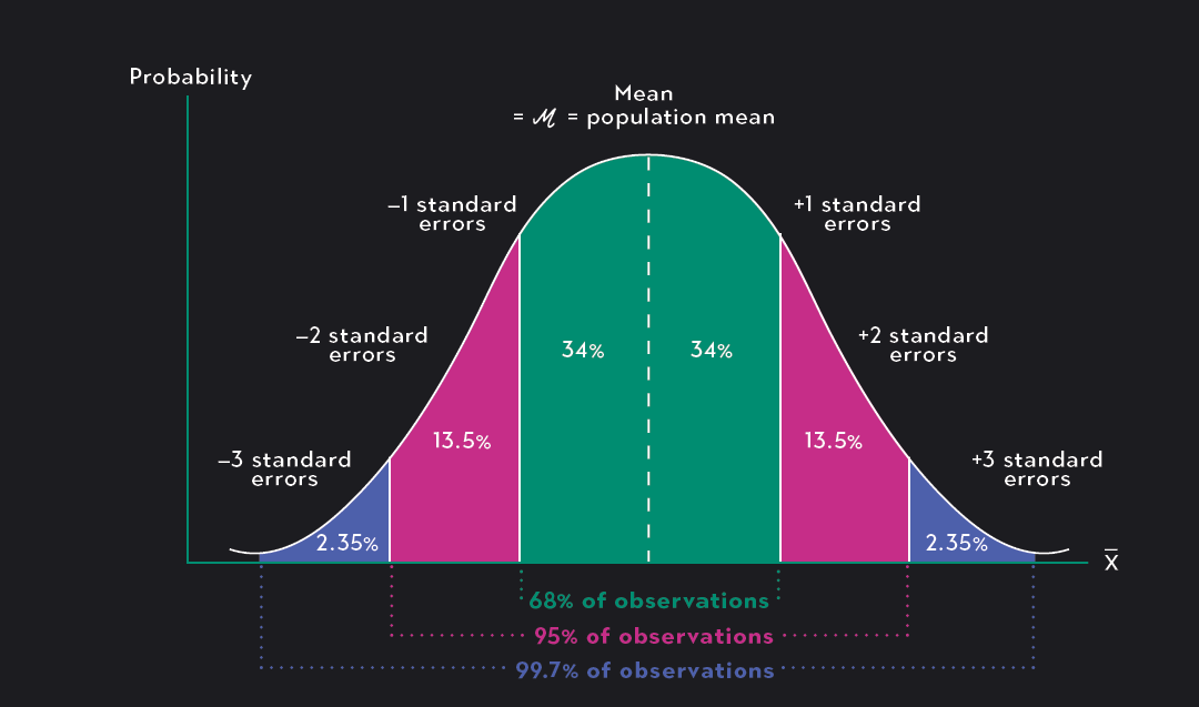
Sampling distributions: as N grows, the spread of estimated means (SE) shrinks
Step 5: Comparing Anna vs Ben — The A/B Test
Now we move from describing one barista to comparing two. This is the heart of A/B testing.
We define the observed difference:
Anna appears 3 seconds faster. But is built from two noisy estimates — so it has its own uncertainty:
%3btext-align:center%3b%7d%23mermaid-6 .edgeLabel p%7bbackground-color:rgba(232%2c232%2c232%2c 0.8)%3b%7d%23mermaid-6 .edgeLabel rect%7bopacity:0.5%3bbackground-color:rgba(232%2c232%2c232%2c 0.8)%3bfill:rgba(232%2c232%2c232%2c 0.8)%3b%7d%23mermaid-6 .labelBkg%7bbackground-color:rgba(232%2c 232%2c 232%2c 0.5)%3b%7d%23mermaid-6 .cluster rect%7bfill:%23ffffde%3bstroke:%23aaaa33%3bstroke-width:1px%3b%7d%23mermaid-6 .cluster text%7bfill:%23333%3b%7d%23mermaid-6 .cluster span%7bcolor:%23333%3b%7d%23mermaid-6 div.mermaidTooltip%7bposition:absolute%3btext-align:center%3bmax-width:200px%3bpadding:2px%3bfont-family:arial%2csans-serif%3bfont-size:12px%3bbackground:hsl(80%2c 100%25%2c 96.2745098039%25)%3bborder:1px solid %23aaaa33%3bborder-radius:2px%3bpointer-events:none%3bz-index:100%3b%7d%23mermaid-6 .flowchartTitleText%7btext-anchor:middle%3bfont-size:18px%3bfill:%23333%3b%7d%23mermaid-6 rect.text%7bfill:none%3bstroke-width:0%3b%7d%23mermaid-6 .icon-shape%2c%23mermaid-6 .image-shape%7bbackground-color:rgba(232%2c232%2c232%2c 0.8)%3btext-align:center%3b%7d%23mermaid-6 .icon-shape p%2c%23mermaid-6 .image-shape p%7bbackground-color:rgba(232%2c232%2c232%2c 0.8)%3bpadding:2px%3b%7d%23mermaid-6 .icon-shape rect%2c%23mermaid-6 .image-shape rect%7bopacity:0.5%3bbackground-color:rgba(232%2c232%2c232%2c 0.8)%3bfill:rgba(232%2c232%2c232%2c 0.8)%3b%7d%23mermaid-6 .label-icon%7bdisplay:inline-block%3bheight:1em%3boverflow:visible%3bvertical-align:-0.125em%3b%7d%23mermaid-6 .node .label-icon path%7bfill:currentColor%3bstroke:revert%3bstroke-width:revert%3b%7d%23mermaid-6 :root%7b--mermaid-font-family:arial%2csans-serif%3b%7d%3c/style%3e%3cg%3e%3cmarker id='mermaid-6_flowchart-v2-pointEnd' class='marker flowchart-v2' viewBox='0 0 10 10' refX='5' refY='5' markerUnits='userSpaceOnUse' markerWidth='8' markerHeight='8' orient='auto'%3e%3cpath d='M 0 0 L 10 5 L 0 10 z' class='arrowMarkerPath' style='stroke-width: 1%3b stroke-dasharray: 1%2c 0%3b'/%3e%3c/marker%3e%3cmarker id='mermaid-6_flowchart-v2-pointStart' class='marker flowchart-v2' viewBox='0 0 10 10' refX='4.5' refY='5' markerUnits='userSpaceOnUse' markerWidth='8' markerHeight='8' orient='auto'%3e%3cpath d='M 0 5 L 10 10 L 10 0 z' class='arrowMarkerPath' style='stroke-width: 1%3b stroke-dasharray: 1%2c 0%3b'/%3e%3c/marker%3e%3cmarker id='mermaid-6_flowchart-v2-circleEnd' class='marker flowchart-v2' viewBox='0 0 10 10' refX='11' refY='5' markerUnits='userSpaceOnUse' markerWidth='11' markerHeight='11' orient='auto'%3e%3ccircle cx='5' cy='5' r='5' class='arrowMarkerPath' style='stroke-width: 1%3b stroke-dasharray: 1%2c 0%3b'/%3e%3c/marker%3e%3cmarker id='mermaid-6_flowchart-v2-circleStart' class='marker flowchart-v2' viewBox='0 0 10 10' refX='-1' refY='5' markerUnits='userSpaceOnUse' markerWidth='11' markerHeight='11' orient='auto'%3e%3ccircle cx='5' cy='5' r='5' class='arrowMarkerPath' style='stroke-width: 1%3b stroke-dasharray: 1%2c 0%3b'/%3e%3c/marker%3e%3cmarker id='mermaid-6_flowchart-v2-crossEnd' class='marker cross flowchart-v2' viewBox='0 0 11 11' refX='12' refY='5.2' markerUnits='userSpaceOnUse' markerWidth='11' markerHeight='11' orient='auto'%3e%3cpath d='M 1%2c1 l 9%2c9 M 10%2c1 l -9%2c9' class='arrowMarkerPath' style='stroke-width: 2%3b stroke-dasharray: 1%2c 0%3b'/%3e%3c/marker%3e%3cmarker id='mermaid-6_flowchart-v2-crossStart' class='marker cross flowchart-v2' viewBox='0 0 11 11' refX='-1' refY='5.2' markerUnits='userSpaceOnUse' markerWidth='11' markerHeight='11' orient='auto'%3e%3cpath d='M 1%2c1 l 9%2c9 M 10%2c1 l -9%2c9' class='arrowMarkerPath' style='stroke-width: 2%3b stroke-dasharray: 1%2c 0%3b'/%3e%3c/marker%3e%3cg class='root'%3e%3cg class='clusters'%3e%3cg class='cluster' id='ben_est' data-look='classic'%3e%3crect style='fill:%231e293b !important%3bstroke:%23ef4444 !important' x='430.78125' y='8' width='402.78125' height='104'/%3e%3cg class='cluster-label' transform='translate(579.0625%2c 8)'%3e%3cforeignObject width='106.21875' height='24'%3e%3cdiv xmlns='http://www.w3.org/1999/xhtml' style='display: table-cell%3b white-space: nowrap%3b line-height: 1.5%3b max-width: 200px%3b text-align: center%3b'%3e%3cspan class='nodeLabel' style='color:%2394a3b8 !important'%3e%3cp%3eBen's Estimate%3c/p%3e%3c/span%3e%3c/div%3e%3c/foreignObject%3e%3c/g%3e%3c/g%3e%3cg class='cluster' id='anna_est' data-look='classic'%3e%3crect style='fill:%231e293b !important%3bstroke:%2322c55e !important' x='8' y='8' width='402.78125' height='104'/%3e%3cg class='cluster-label' transform='translate(151.8359375%2c 8)'%3e%3cforeignObject width='115.109375' height='24'%3e%3cdiv xmlns='http://www.w3.org/1999/xhtml' style='display: table-cell%3b white-space: nowrap%3b line-height: 1.5%3b max-width: 200px%3b text-align: center%3b'%3e%3cspan class='nodeLabel' style='color:%2394a3b8 !important'%3e%3cp%3eAnna's Estimate%3c/p%3e%3c/span%3e%3c/div%3e%3c/foreignObject%3e%3c/g%3e%3c/g%3e%3c/g%3e%3cg class='edgePaths'%3e%3cpath d='M306.422%2c87L306.422%2c91.167C306.422%2c95.333%2c306.422%2c103.667%2c327.371%2c112C348.32%2c120.333%2c390.219%2c128.667%2c436.698%2c138.525C483.178%2c148.383%2c534.238%2c159.766%2c559.769%2c165.457L585.299%2c171.149' id='L_ASE_SE_D_0' class='edge-thickness-normal edge-pattern-solid edge-thickness-normal edge-pattern-solid flowchart-link' style='%3b' data-edge='true' data-et='edge' data-id='L_ASE_SE_D_0' data-points='W3sieCI6MzA2LjQyMTg3NSwieSI6ODd9LHsieCI6MzA2LjQyMTg3NSwieSI6MTEyfSx7IngiOjQzMi4xMTcxODc1LCJ5IjoxMzd9LHsieCI6NTg5LjIwMzEyNSwieSI6MTcyLjAxOTEzMDgxMzM5OTczfV0=' marker-end='url(%23mermaid-6_flowchart-v2-pointEnd)'/%3e%3cpath d='M729.203%2c87L729.203%2c91.167C729.203%2c95.333%2c729.203%2c103.667%2c729.203%2c112C729.203%2c120.333%2c729.203%2c128.667%2c728.655%2c136.341C728.107%2c144.016%2c727.011%2c151.032%2c726.463%2c154.54L725.914%2c158.048' id='L_BSE_SE_D_0' class='edge-thickness-normal edge-pattern-solid edge-thickness-normal edge-pattern-solid flowchart-link' style='%3b' data-edge='true' data-et='edge' data-id='L_BSE_SE_D_0' data-points='W3sieCI6NzI5LjIwMzEyNSwieSI6ODd9LHsieCI6NzI5LjIwMzEyNSwieSI6MTEyfSx7IngiOjcyOS4yMDMxMjUsInkiOjEzN30seyJ4Ijo3MjUuMjk2ODc1LCJ5IjoxNjJ9XQ==' marker-end='url(%23mermaid-6_flowchart-v2-pointEnd)'/%3e%3cpath d='M125.031%2c228L125.031%2c234.167C125.031%2c240.333%2c125.031%2c252.667%2c160.802%2c275.855C196.572%2c299.044%2c268.113%2c333.089%2c303.883%2c350.111L339.654%2c367.133' id='L_DELTA_QUESTION_0' class='edge-thickness-normal edge-pattern-solid edge-thickness-normal edge-pattern-solid flowchart-link' style='%3b' data-edge='true' data-et='edge' data-id='L_DELTA_QUESTION_0' data-points='W3sieCI6MTI1LjAzMTI1LCJ5IjoyMjh9LHsieCI6MTI1LjAzMTI1LCJ5IjoyNjV9LHsieCI6MzQzLjI2NTUyMDE4MDAwNjQzLCJ5IjozNjguODUxNjY3MzE5OTkzNTd9XQ==' marker-end='url(%23mermaid-6_flowchart-v2-pointEnd)'/%3e%3cpath d='M719.203%2c240L719.203%2c244.167C719.203%2c248.333%2c719.203%2c256.667%2c683.433%2c277.855C647.662%2c299.044%2c576.122%2c333.089%2c540.351%2c350.111L504.581%2c367.133' id='L_SE_D_QUESTION_0' class='edge-thickness-normal edge-pattern-solid edge-thickness-normal edge-pattern-solid flowchart-link' style='%3b' data-edge='true' data-et='edge' data-id='L_SE_D_QUESTION_0' data-points='W3sieCI6NzE5LjIwMzEyNSwieSI6MjQwfSx7IngiOjcxOS4yMDMxMjUsInkiOjI2NX0seyJ4Ijo1MDAuOTY4ODU0ODE5OTkzNTcsInkiOjM2OC44NTE2NjczMTk5OTM1N31d' marker-end='url(%23mermaid-6_flowchart-v2-pointEnd)'/%3e%3cpath d='M115.031%2c112L115.031%2c116.167C115.031%2c120.333%2c115.031%2c128.667%2c115.892%2c138.341C116.752%2c148.016%2c118.474%2c159.032%2c119.334%2c164.54L120.195%2c170.048' id='L_anna_est_DELTA_0' class='edge-thickness-normal edge-pattern-solid edge-thickness-normal edge-pattern-solid flowchart-link' style='%3b' data-edge='true' data-et='edge' data-id='L_anna_est_DELTA_0' data-points='W3sieCI6MTE1LjAzMTI1LCJ5Ijo4N30seyJ4IjoxMTUuMDMxMjUsInkiOjExMn0seyJ4IjoxMTUuMDMxMjUsInkiOjEzN30seyJ4IjoxMjAuODEyNSwieSI6MTc0fV0=' marker-end='url(%23mermaid-6_flowchart-v2-pointEnd)'/%3e%3cpath d='M537.813%2c112L516.863%2c116.167C495.914%2c120.333%2c454.016%2c128.667%2c400.655%2c140.059C347.294%2c151.451%2c282.47%2c165.902%2c250.058%2c173.128L217.646%2c180.353' id='L_ben_est_DELTA_0' class='edge-thickness-normal edge-pattern-solid edge-thickness-normal edge-pattern-solid flowchart-link' style='%3b' data-edge='true' data-et='edge' data-id='L_ben_est_DELTA_0' data-points='W3sieCI6NTM3LjgxMjUsInkiOjg3fSx7IngiOjUzNy44MTI1LCJ5IjoxMTJ9LHsieCI6NDEyLjExNzE4NzUsInkiOjEzN30seyJ4IjoyMTMuNzQyMTg3NSwieSI6MTgxLjIyMzY5MTcyOTkzNzE0fV0=' marker-end='url(%23mermaid-6_flowchart-v2-pointEnd)'/%3e%3c/g%3e%3cg class='edgeLabels'%3e%3cg class='edgeLabel'%3e%3cg class='label' data-id='L_ASE_SE_D_0' transform='translate(0%2c 0)'%3e%3cforeignObject width='0' height='0'%3e%3cdiv xmlns='http://www.w3.org/1999/xhtml' class='labelBkg' style='display: table-cell%3b white-space: nowrap%3b line-height: 1.5%3b max-width: 200px%3b text-align: center%3b'%3e%3cspan class='edgeLabel'%3e%3c/span%3e%3c/div%3e%3c/foreignObject%3e%3c/g%3e%3c/g%3e%3cg class='edgeLabel'%3e%3cg class='label' data-id='L_BSE_SE_D_0' transform='translate(0%2c 0)'%3e%3cforeignObject width='0' height='0'%3e%3cdiv xmlns='http://www.w3.org/1999/xhtml' class='labelBkg' style='display: table-cell%3b white-space: nowrap%3b line-height: 1.5%3b max-width: 200px%3b text-align: center%3b'%3e%3cspan class='edgeLabel'%3e%3c/span%3e%3c/div%3e%3c/foreignObject%3e%3c/g%3e%3c/g%3e%3cg class='edgeLabel'%3e%3cg class='label' data-id='L_DELTA_QUESTION_0' transform='translate(0%2c 0)'%3e%3cforeignObject width='0' height='0'%3e%3cdiv xmlns='http://www.w3.org/1999/xhtml' class='labelBkg' style='display: table-cell%3b white-space: nowrap%3b line-height: 1.5%3b max-width: 200px%3b text-align: center%3b'%3e%3cspan class='edgeLabel'%3e%3c/span%3e%3c/div%3e%3c/foreignObject%3e%3c/g%3e%3c/g%3e%3cg class='edgeLabel'%3e%3cg class='label' data-id='L_SE_D_QUESTION_0' transform='translate(0%2c 0)'%3e%3cforeignObject width='0' height='0'%3e%3cdiv xmlns='http://www.w3.org/1999/xhtml' class='labelBkg' style='display: table-cell%3b white-space: nowrap%3b line-height: 1.5%3b max-width: 200px%3b text-align: center%3b'%3e%3cspan class='edgeLabel'%3e%3c/span%3e%3c/div%3e%3c/foreignObject%3e%3c/g%3e%3c/g%3e%3cg class='edgeLabel'%3e%3cg class='label' data-id='L_anna_est_DELTA_0' transform='translate(0%2c 0)'%3e%3cforeignObject width='0' height='0'%3e%3cdiv xmlns='http://www.w3.org/1999/xhtml' class='labelBkg' style='display: table-cell%3b white-space: nowrap%3b line-height: 1.5%3b max-width: 200px%3b text-align: center%3b'%3e%3cspan class='edgeLabel'%3e%3c/span%3e%3c/div%3e%3c/foreignObject%3e%3c/g%3e%3c/g%3e%3cg class='edgeLabel'%3e%3cg class='label' data-id='L_ben_est_DELTA_0' transform='translate(0%2c 0)'%3e%3cforeignObject width='0' height='0'%3e%3cdiv xmlns='http://www.w3.org/1999/xhtml' class='labelBkg' style='display: table-cell%3b white-space: nowrap%3b line-height: 1.5%3b max-width: 200px%3b text-align: center%3b'%3e%3cspan class='edgeLabel'%3e%3c/span%3e%3c/div%3e%3c/foreignObject%3e%3c/g%3e%3c/g%3e%3c/g%3e%3cg class='nodes'%3e%3cg class='node default' id='flowchart-AM-0' transform='translate(115.03125%2c 60)'%3e%3crect class='basic label-container' style='' x='-72.03125' y='-27' width='144.0625' height='54'/%3e%3cg class='label' style='' transform='translate(-42.03125%2c -12)'%3e%3crect/%3e%3cforeignObject width='84.0625' height='24'%3e%3cdiv xmlns='http://www.w3.org/1999/xhtml' style='display: table-cell%3b white-space: nowrap%3b line-height: 1.5%3b max-width: 200px%3b text-align: center%3b'%3e%3cspan class='nodeLabel'%3e%3cp%3eMean = 28s%3c/p%3e%3c/span%3e%3c/div%3e%3c/foreignObject%3e%3c/g%3e%3c/g%3e%3cg class='node default' id='flowchart-ASE-1' transform='translate(306.421875%2c 60)'%3e%3crect class='basic label-container' style='' x='-69.359375' y='-27' width='138.71875' height='54'/%3e%3cg class='label' style='' transform='translate(-39.359375%2c -12)'%3e%3crect/%3e%3cforeignObject width='78.71875' height='24'%3e%3cdiv xmlns='http://www.w3.org/1999/xhtml' style='display: table-cell%3b white-space: nowrap%3b line-height: 1.5%3b max-width: 200px%3b text-align: center%3b'%3e%3cspan class='nodeLabel'%3e%3cp%3eSE = 0.85s%3c/p%3e%3c/span%3e%3c/div%3e%3c/foreignObject%3e%3c/g%3e%3c/g%3e%3cg class='node default' id='flowchart-BM-2' transform='translate(537.8125%2c 60)'%3e%3crect class='basic label-container' style='' x='-72.03125' y='-27' width='144.0625' height='54'/%3e%3cg class='label' style='' transform='translate(-42.03125%2c -12)'%3e%3crect/%3e%3cforeignObject width='84.0625' height='24'%3e%3cdiv xmlns='http://www.w3.org/1999/xhtml' style='display: table-cell%3b white-space: nowrap%3b line-height: 1.5%3b max-width: 200px%3b text-align: center%3b'%3e%3cspan class='nodeLabel'%3e%3cp%3eMean = 31s%3c/p%3e%3c/span%3e%3c/div%3e%3c/foreignObject%3e%3c/g%3e%3c/g%3e%3cg class='node default' id='flowchart-BSE-3' transform='translate(729.203125%2c 60)'%3e%3crect class='basic label-container' style='' x='-69.359375' y='-27' width='138.71875' height='54'/%3e%3cg class='label' style='' transform='translate(-39.359375%2c -12)'%3e%3crect/%3e%3cforeignObject width='78.71875' height='24'%3e%3cdiv xmlns='http://www.w3.org/1999/xhtml' style='display: table-cell%3b white-space: nowrap%3b line-height: 1.5%3b max-width: 200px%3b text-align: center%3b'%3e%3cspan class='nodeLabel'%3e%3cp%3eSE = 1.70s%3c/p%3e%3c/span%3e%3c/div%3e%3c/foreignObject%3e%3c/g%3e%3c/g%3e%3cg class='node default' id='flowchart-DELTA-5' transform='translate(125.03125%2c 201)'%3e%3crect class='basic label-container' style='fill:%23a855f7 !important%3bstroke:none !important' x='-88.7109375' y='-27' width='177.421875' height='54'/%3e%3cg class='label' style='color:white !important' transform='translate(-58.7109375%2c -12)'%3e%3crect/%3e%3cforeignObject width='117.421875' height='24'%3e%3cdiv style='color: rgb(255%2c 255%2c 255) !important%3b display: table-cell%3b white-space: nowrap%3b line-height: 1.5%3b max-width: 200px%3b text-align: center%3b' xmlns='http://www.w3.org/1999/xhtml'%3e%3cspan style='color:white !important' class='nodeLabel'%3e%3cp%3e%ce%b4 = 28 - 31 = -3s%3c/p%3e%3c/span%3e%3c/div%3e%3c/foreignObject%3e%3c/g%3e%3c/g%3e%3cg class='node default' id='flowchart-SE_D-9' transform='translate(719.203125%2c 201)'%3e%3crect class='basic label-container' style='fill:%23f97316 !important%3bstroke:none !important' x='-130' y='-39' width='260' height='78'/%3e%3cg class='label' style='color:white !important' transform='translate(-100%2c -24)'%3e%3crect/%3e%3cforeignObject width='200' height='48'%3e%3cdiv style='color: rgb(255%2c 255%2c 255) !important%3b display: table%3b white-space: break-spaces%3b line-height: 1.5%3b max-width: 200px%3b text-align: center%3b width: 200px%3b' xmlns='http://www.w3.org/1999/xhtml'%3e%3cspan style='color:white !important' class='nodeLabel'%3e%3cp%3eSE_%ce%b4 = %e2%88%9a(0.85%c2%b2 %2b 1.70%c2%b2)%5cn= 1.90s%3c/p%3e%3c/span%3e%3c/div%3e%3c/foreignObject%3e%3c/g%3e%3c/g%3e%3cg class='node default' id='flowchart-QUESTION-13' transform='translate(422.1171875%2c 406.375)'%3e%3cpolygon points='116.375%2c0 232.75%2c-116.375 116.375%2c-232.75 0%2c-116.375' class='label-container' transform='translate(-115.875%2c 116.375)' style='fill:%23f59e0b !important%3bstroke:none !important'/%3e%3cg class='label' style='color:black !important' transform='translate(-89.375%2c -12)'%3e%3crect/%3e%3cforeignObject width='178.75' height='24'%3e%3cdiv style='color: rgb(0%2c 0%2c 0) !important%3b display: table-cell%3b white-space: nowrap%3b line-height: 1.5%3b max-width: 200px%3b text-align: center%3b' xmlns='http://www.w3.org/1999/xhtml'%3e%3cspan style='color:black !important' class='nodeLabel'%3e%3cp%3eIs -3s real%5cnor just noise%3f%3c/p%3e%3c/span%3e%3c/div%3e%3c/foreignObject%3e%3c/g%3e%3c/g%3e%3c/g%3e%3c/g%3e%3c/g%3e%3c/svg%3e)
Caveat
The variance-addition rule () only holds when the two groups are independent. In a proper A/B test where users are randomly assigned, this is guaranteed. In observational data, it may not be.
Step 6: The z-Score — Signal vs Noise
We compress the entire comparison into a single number:
- z-score
-
How many standard errors the observed difference is from zero. It’s the ratio of signal (the difference you saw) to noise (the uncertainty in that difference).
%3btext-align:center%3b%7d%23mermaid-7 .edgeLabel p%7bbackground-color:rgba(232%2c232%2c232%2c 0.8)%3b%7d%23mermaid-7 .edgeLabel rect%7bopacity:0.5%3bbackground-color:rgba(232%2c232%2c232%2c 0.8)%3bfill:rgba(232%2c232%2c232%2c 0.8)%3b%7d%23mermaid-7 .labelBkg%7bbackground-color:rgba(232%2c 232%2c 232%2c 0.5)%3b%7d%23mermaid-7 .cluster rect%7bfill:%23ffffde%3bstroke:%23aaaa33%3bstroke-width:1px%3b%7d%23mermaid-7 .cluster text%7bfill:%23333%3b%7d%23mermaid-7 .cluster span%7bcolor:%23333%3b%7d%23mermaid-7 div.mermaidTooltip%7bposition:absolute%3btext-align:center%3bmax-width:200px%3bpadding:2px%3bfont-family:arial%2csans-serif%3bfont-size:12px%3bbackground:hsl(80%2c 100%25%2c 96.2745098039%25)%3bborder:1px solid %23aaaa33%3bborder-radius:2px%3bpointer-events:none%3bz-index:100%3b%7d%23mermaid-7 .flowchartTitleText%7btext-anchor:middle%3bfont-size:18px%3bfill:%23333%3b%7d%23mermaid-7 rect.text%7bfill:none%3bstroke-width:0%3b%7d%23mermaid-7 .icon-shape%2c%23mermaid-7 .image-shape%7bbackground-color:rgba(232%2c232%2c232%2c 0.8)%3btext-align:center%3b%7d%23mermaid-7 .icon-shape p%2c%23mermaid-7 .image-shape p%7bbackground-color:rgba(232%2c232%2c232%2c 0.8)%3bpadding:2px%3b%7d%23mermaid-7 .icon-shape rect%2c%23mermaid-7 .image-shape rect%7bopacity:0.5%3bbackground-color:rgba(232%2c232%2c232%2c 0.8)%3bfill:rgba(232%2c232%2c232%2c 0.8)%3b%7d%23mermaid-7 .label-icon%7bdisplay:inline-block%3bheight:1em%3boverflow:visible%3bvertical-align:-0.125em%3b%7d%23mermaid-7 .node .label-icon path%7bfill:currentColor%3bstroke:revert%3bstroke-width:revert%3b%7d%23mermaid-7 :root%7b--mermaid-font-family:arial%2csans-serif%3b%7d%3c/style%3e%3cg%3e%3cmarker id='mermaid-7_flowchart-v2-pointEnd' class='marker flowchart-v2' viewBox='0 0 10 10' refX='5' refY='5' markerUnits='userSpaceOnUse' markerWidth='8' markerHeight='8' orient='auto'%3e%3cpath d='M 0 0 L 10 5 L 0 10 z' class='arrowMarkerPath' style='stroke-width: 1%3b stroke-dasharray: 1%2c 0%3b'/%3e%3c/marker%3e%3cmarker id='mermaid-7_flowchart-v2-pointStart' class='marker flowchart-v2' viewBox='0 0 10 10' refX='4.5' refY='5' markerUnits='userSpaceOnUse' markerWidth='8' markerHeight='8' orient='auto'%3e%3cpath d='M 0 5 L 10 10 L 10 0 z' class='arrowMarkerPath' style='stroke-width: 1%3b stroke-dasharray: 1%2c 0%3b'/%3e%3c/marker%3e%3cmarker id='mermaid-7_flowchart-v2-circleEnd' class='marker flowchart-v2' viewBox='0 0 10 10' refX='11' refY='5' markerUnits='userSpaceOnUse' markerWidth='11' markerHeight='11' orient='auto'%3e%3ccircle cx='5' cy='5' r='5' class='arrowMarkerPath' style='stroke-width: 1%3b stroke-dasharray: 1%2c 0%3b'/%3e%3c/marker%3e%3cmarker id='mermaid-7_flowchart-v2-circleStart' class='marker flowchart-v2' viewBox='0 0 10 10' refX='-1' refY='5' markerUnits='userSpaceOnUse' markerWidth='11' markerHeight='11' orient='auto'%3e%3ccircle cx='5' cy='5' r='5' class='arrowMarkerPath' style='stroke-width: 1%3b stroke-dasharray: 1%2c 0%3b'/%3e%3c/marker%3e%3cmarker id='mermaid-7_flowchart-v2-crossEnd' class='marker cross flowchart-v2' viewBox='0 0 11 11' refX='12' refY='5.2' markerUnits='userSpaceOnUse' markerWidth='11' markerHeight='11' orient='auto'%3e%3cpath d='M 1%2c1 l 9%2c9 M 10%2c1 l -9%2c9' class='arrowMarkerPath' style='stroke-width: 2%3b stroke-dasharray: 1%2c 0%3b'/%3e%3c/marker%3e%3cmarker id='mermaid-7_flowchart-v2-crossStart' class='marker cross flowchart-v2' viewBox='0 0 11 11' refX='-1' refY='5.2' markerUnits='userSpaceOnUse' markerWidth='11' markerHeight='11' orient='auto'%3e%3cpath d='M 1%2c1 l 9%2c9 M 10%2c1 l -9%2c9' class='arrowMarkerPath' style='stroke-width: 2%3b stroke-dasharray: 1%2c 0%3b'/%3e%3c/marker%3e%3cg class='root'%3e%3cg class='clusters'/%3e%3cg class='edgePaths'%3e%3cpath d='M188.078%2c99L194.393%2c99C200.708%2c99%2c213.339%2c99%2c225.48%2c100.955C237.621%2c102.909%2c249.274%2c106.819%2c255.1%2c108.773L260.926%2c110.728' id='L_SIG_Z_0' class='edge-thickness-normal edge-pattern-solid edge-thickness-normal edge-pattern-solid flowchart-link' style='%3b' data-edge='true' data-et='edge' data-id='L_SIG_Z_0' data-points='W3sieCI6MTg4LjA3ODEyNSwieSI6OTl9LHsieCI6MjI1Ljk2ODc1LCJ5Ijo5OX0seyJ4IjoyNjQuNzE4NzUsInkiOjExMn1d' marker-end='url(%23mermaid-7_flowchart-v2-pointEnd)'/%3e%3cpath d='M200.969%2c203L205.135%2c203C209.302%2c203%2c217.635%2c203%2c227.628%2c201.045C237.621%2c199.091%2c249.274%2c195.181%2c255.1%2c193.227L260.926%2c191.272' id='L_NOISE_Z_0' class='edge-thickness-normal edge-pattern-solid edge-thickness-normal edge-pattern-solid flowchart-link' style='%3b' data-edge='true' data-et='edge' data-id='L_NOISE_Z_0' data-points='W3sieCI6MjAwLjk2ODc1LCJ5IjoyMDN9LHsieCI6MjI1Ljk2ODc1LCJ5IjoyMDN9LHsieCI6MjY0LjcxODc1LCJ5IjoxOTB9XQ==' marker-end='url(%23mermaid-7_flowchart-v2-pointEnd)'/%3e%3cpath d='M510.969%2c151L515.135%2c151C519.302%2c151%2c527.635%2c151%2c535.302%2c151C542.969%2c151%2c549.969%2c151%2c553.469%2c151L556.969%2c151' id='L_Z_INT_0' class='edge-thickness-normal edge-pattern-solid edge-thickness-normal edge-pattern-solid flowchart-link' style='%3b' data-edge='true' data-et='edge' data-id='L_Z_INT_0' data-points='W3sieCI6NTEwLjk2ODc1LCJ5IjoxNTF9LHsieCI6NTM1Ljk2ODc1LCJ5IjoxNTF9LHsieCI6NTYwLjk2ODc1LCJ5IjoxNTF9XQ==' marker-end='url(%23mermaid-7_flowchart-v2-pointEnd)'/%3e%3cpath d='M674.569%2c116.319L689.99%2c102.766C705.411%2c89.213%2c736.252%2c62.106%2c761.475%2c48.553C786.698%2c35%2c806.302%2c35%2c816.104%2c35L825.906%2c35' id='L_INT_NO_0' class='edge-thickness-normal edge-pattern-solid edge-thickness-normal edge-pattern-solid flowchart-link' style='%3b' data-edge='true' data-et='edge' data-id='L_INT_NO_0' data-points='W3sieCI6Njc0LjU2OTEzNTUzMDIxMjMsInkiOjExNi4zMTkxMzU1MzAyMTIzNH0seyJ4Ijo3NjcuMDkzNzUsInkiOjM1fSx7IngiOjgyOS45MDYyNSwieSI6MzV9XQ==' marker-end='url(%23mermaid-7_flowchart-v2-pointEnd)'/%3e%3cpath d='M709.25%2c151L718.891%2c151C728.531%2c151%2c747.813%2c151%2c766.427%2c151C785.042%2c151%2c802.99%2c151%2c811.964%2c151L820.938%2c151' id='L_INT_YES_0' class='edge-thickness-normal edge-pattern-solid edge-thickness-normal edge-pattern-solid flowchart-link' style='%3b' data-edge='true' data-et='edge' data-id='L_INT_YES_0' data-points='W3sieCI6NzA5LjI1LCJ5IjoxNTF9LHsieCI6NzY3LjA5Mzc1LCJ5IjoxNTF9LHsieCI6ODI0LjkzNzUsInkiOjE1MX1d' marker-end='url(%23mermaid-7_flowchart-v2-pointEnd)'/%3e%3cpath d='M672.748%2c187.502L688.472%2c202.752C704.196%2c218.001%2c735.645%2c248.501%2c760.343%2c263.75C785.042%2c279%2c802.99%2c279%2c811.964%2c279L820.938%2c279' id='L_INT_MAYBE_0' class='edge-thickness-normal edge-pattern-solid edge-thickness-normal edge-pattern-solid flowchart-link' style='%3b' data-edge='true' data-et='edge' data-id='L_INT_MAYBE_0' data-points='W3sieCI6NjcyLjc0NzgwNjM1ODU1NTIsInkiOjE4Ny41MDIxOTM2NDE0NDQ4fSx7IngiOjc2Ny4wOTM3NSwieSI6Mjc5fSx7IngiOjgyNC45Mzc1LCJ5IjoyNzl9XQ==' marker-end='url(%23mermaid-7_flowchart-v2-pointEnd)'/%3e%3c/g%3e%3cg class='edgeLabels'%3e%3cg class='edgeLabel'%3e%3cg class='label' data-id='L_SIG_Z_0' transform='translate(0%2c 0)'%3e%3cforeignObject width='0' height='0'%3e%3cdiv xmlns='http://www.w3.org/1999/xhtml' class='labelBkg' style='display: table-cell%3b white-space: nowrap%3b line-height: 1.5%3b max-width: 200px%3b text-align: center%3b'%3e%3cspan class='edgeLabel'%3e%3c/span%3e%3c/div%3e%3c/foreignObject%3e%3c/g%3e%3c/g%3e%3cg class='edgeLabel'%3e%3cg class='label' data-id='L_NOISE_Z_0' transform='translate(0%2c 0)'%3e%3cforeignObject width='0' height='0'%3e%3cdiv xmlns='http://www.w3.org/1999/xhtml' class='labelBkg' style='display: table-cell%3b white-space: nowrap%3b line-height: 1.5%3b max-width: 200px%3b text-align: center%3b'%3e%3cspan class='edgeLabel'%3e%3c/span%3e%3c/div%3e%3c/foreignObject%3e%3c/g%3e%3c/g%3e%3cg class='edgeLabel'%3e%3cg class='label' data-id='L_Z_INT_0' transform='translate(0%2c 0)'%3e%3cforeignObject width='0' height='0'%3e%3cdiv xmlns='http://www.w3.org/1999/xhtml' class='labelBkg' style='display: table-cell%3b white-space: nowrap%3b line-height: 1.5%3b max-width: 200px%3b text-align: center%3b'%3e%3cspan class='edgeLabel'%3e%3c/span%3e%3c/div%3e%3c/foreignObject%3e%3c/g%3e%3c/g%3e%3cg class='edgeLabel' transform='translate(767.09375%2c 35)'%3e%3cg class='label' data-id='L_INT_NO_0' transform='translate(-28.90625%2c -12)'%3e%3cforeignObject width='57.8125' height='24'%3e%3cdiv xmlns='http://www.w3.org/1999/xhtml' class='labelBkg' style='display: table-cell%3b white-space: nowrap%3b line-height: 1.5%3b max-width: 200px%3b text-align: center%3b'%3e%3cspan class='edgeLabel'%3e%3cp%3ez near 0%3c/p%3e%3c/span%3e%3c/div%3e%3c/foreignObject%3e%3c/g%3e%3c/g%3e%3cg class='edgeLabel' transform='translate(767.09375%2c 151)'%3e%3cg class='label' data-id='L_INT_YES_0' transform='translate(-21.7265625%2c -12)'%3e%3cforeignObject width='43.453125' height='24'%3e%3cdiv xmlns='http://www.w3.org/1999/xhtml' class='labelBkg' style='display: table-cell%3b white-space: nowrap%3b line-height: 1.5%3b max-width: 200px%3b text-align: center%3b'%3e%3cspan class='edgeLabel'%3e%3cp%3e%7cz%7c %26gt%3b 2%3c/p%3e%3c/span%3e%3c/div%3e%3c/foreignObject%3e%3c/g%3e%3c/g%3e%3cg class='edgeLabel' transform='translate(767.09375%2c 279)'%3e%3cg class='label' data-id='L_INT_MAYBE_0' transform='translate(-32.84375%2c -12)'%3e%3cforeignObject width='65.6875' height='24'%3e%3cdiv xmlns='http://www.w3.org/1999/xhtml' class='labelBkg' style='display: table-cell%3b white-space: nowrap%3b line-height: 1.5%3b max-width: 200px%3b text-align: center%3b'%3e%3cspan class='edgeLabel'%3e%3cp%3e%7cz%7c = 1.58%3c/p%3e%3c/span%3e%3c/div%3e%3c/foreignObject%3e%3c/g%3e%3c/g%3e%3c/g%3e%3cg class='nodes'%3e%3cg class='node default' id='flowchart-SIG-0' transform='translate(104.484375%2c 99)'%3e%3crect class='basic label-container' style='fill:%2322c55e !important%3bstroke:none !important' x='-83.59375' y='-27' width='167.1875' height='54'/%3e%3cg class='label' style='color:white !important' transform='translate(-53.59375%2c -12)'%3e%3crect/%3e%3cforeignObject width='107.1875' height='24'%3e%3cdiv style='color: rgb(255%2c 255%2c 255) !important%3b display: table-cell%3b white-space: nowrap%3b line-height: 1.5%3b max-width: 200px%3b text-align: center%3b' xmlns='http://www.w3.org/1999/xhtml'%3e%3cspan style='color:white !important' class='nodeLabel'%3e%3cp%3eSignal%5cn%ce%b4 = -3s%3c/p%3e%3c/span%3e%3c/div%3e%3c/foreignObject%3e%3c/g%3e%3c/g%3e%3cg class='node default' id='flowchart-Z-1' transform='translate(380.96875%2c 151)'%3e%3crect class='basic label-container' style='fill:%23a855f7 !important%3bstroke:none !important' x='-130' y='-39' width='260' height='78'/%3e%3cg class='label' style='color:white !important' transform='translate(-100%2c -24)'%3e%3crect/%3e%3cforeignObject width='200' height='48'%3e%3cdiv style='color: rgb(255%2c 255%2c 255) !important%3b display: table%3b white-space: break-spaces%3b line-height: 1.5%3b max-width: 200px%3b text-align: center%3b width: 200px%3b' xmlns='http://www.w3.org/1999/xhtml'%3e%3cspan style='color:white !important' class='nodeLabel'%3e%3cp%3ez = signal / noise%5cn= -3 / 1.90%5cn= -1.58%3c/p%3e%3c/span%3e%3c/div%3e%3c/foreignObject%3e%3c/g%3e%3c/g%3e%3cg class='node default' id='flowchart-NOISE-2' transform='translate(104.484375%2c 203)'%3e%3crect class='basic label-container' style='fill:%23ef4444 !important%3bstroke:none !important' x='-96.484375' y='-27' width='192.96875' height='54'/%3e%3cg class='label' style='color:white !important' transform='translate(-66.484375%2c -12)'%3e%3crect/%3e%3cforeignObject width='132.96875' height='24'%3e%3cdiv style='color: rgb(255%2c 255%2c 255) !important%3b display: table-cell%3b white-space: nowrap%3b line-height: 1.5%3b max-width: 200px%3b text-align: center%3b' xmlns='http://www.w3.org/1999/xhtml'%3e%3cspan style='color:white !important' class='nodeLabel'%3e%3cp%3eNoise%5cnSE = 1.90s%3c/p%3e%3c/span%3e%3c/div%3e%3c/foreignObject%3e%3c/g%3e%3c/g%3e%3cg class='node default' id='flowchart-INT-5' transform='translate(635.109375%2c 151)'%3e%3cpolygon points='74.140625%2c0 148.28125%2c-74.140625 74.140625%2c-148.28125 0%2c-74.140625' class='label-container' transform='translate(-73.640625%2c 74.140625)'/%3e%3cg class='label' style='' transform='translate(-47.140625%2c -12)'%3e%3crect/%3e%3cforeignObject width='94.28125' height='24'%3e%3cdiv xmlns='http://www.w3.org/1999/xhtml' style='display: table-cell%3b white-space: nowrap%3b line-height: 1.5%3b max-width: 200px%3b text-align: center%3b'%3e%3cspan class='nodeLabel'%3e%3cp%3eInterpretation%3c/p%3e%3c/span%3e%3c/div%3e%3c/foreignObject%3e%3c/g%3e%3c/g%3e%3cg class='node default' id='flowchart-NO-7' transform='translate(954.9375%2c 35)'%3e%3crect class='basic label-container' style='fill:%2364748b !important%3bstroke:none !important' x='-125.03125' y='-27' width='250.0625' height='54'/%3e%3cg class='label' style='color:white !important' transform='translate(-95.03125%2c -12)'%3e%3crect/%3e%3cforeignObject width='190.0625' height='24'%3e%3cdiv style='color: rgb(255%2c 255%2c 255) !important%3b display: table-cell%3b white-space: nowrap%3b line-height: 1.5%3b max-width: 200px%3b text-align: center%3b' xmlns='http://www.w3.org/1999/xhtml'%3e%3cspan style='color:white !important' class='nodeLabel'%3e%3cp%3eNo evidence%5cnof difference%3c/p%3e%3c/span%3e%3c/div%3e%3c/foreignObject%3e%3c/g%3e%3c/g%3e%3cg class='node default' id='flowchart-YES-9' transform='translate(954.9375%2c 151)'%3e%3crect class='basic label-container' style='fill:%2322c55e !important%3bstroke:none !important' x='-130' y='-39' width='260' height='78'/%3e%3cg class='label' style='color:white !important' transform='translate(-100%2c -24)'%3e%3crect/%3e%3cforeignObject width='200' height='48'%3e%3cdiv style='color: rgb(255%2c 255%2c 255) !important%3b display: table%3b white-space: break-spaces%3b line-height: 1.5%3b max-width: 200px%3b text-align: center%3b width: 200px%3b' xmlns='http://www.w3.org/1999/xhtml'%3e%3cspan style='color:white !important' class='nodeLabel'%3e%3cp%3eStrong evidence%5cnof difference%3c/p%3e%3c/span%3e%3c/div%3e%3c/foreignObject%3e%3c/g%3e%3c/g%3e%3cg class='node default' id='flowchart-MAYBE-11' transform='translate(954.9375%2c 279)'%3e%3crect class='basic label-container' style='fill:%23f97316 !important%3bstroke:none !important' x='-130' y='-39' width='260' height='78'/%3e%3cg class='label' style='color:white !important' transform='translate(-100%2c -24)'%3e%3crect/%3e%3cforeignObject width='200' height='48'%3e%3cdiv style='color: rgb(255%2c 255%2c 255) !important%3b display: table%3b white-space: break-spaces%3b line-height: 1.5%3b max-width: 200px%3b text-align: center%3b width: 200px%3b' xmlns='http://www.w3.org/1999/xhtml'%3e%3cspan style='color:white !important' class='nodeLabel'%3e%3cp%3eSuggestive but%5cnnot conclusive%3c/p%3e%3c/span%3e%3c/div%3e%3c/foreignObject%3e%3c/g%3e%3c/g%3e%3c/g%3e%3c/g%3e%3c/g%3e%3c/svg%3e)
The z-score works because of the Central Limit Theorem: averages of many observations are approximately normally distributed, regardless of the underlying data shape. Dividing by SE standardises this to a known scale:
Quick reference:
| z-score | Meaning |
|---|---|
| 0 | No difference observed |
| ±1 | ~68% of random variation falls within this |
| ±1.96 | The conventional “significance” threshold |
| ±2.5+ | Strong evidence |
Step 7: Hypothesis Testing — Making the Call
We now have all the ingredients. Hypothesis testing wraps them into a decision framework.
%3btext-align:center%3b%7d%23mermaid-8 .edgeLabel p%7bbackground-color:rgba(232%2c232%2c232%2c 0.8)%3b%7d%23mermaid-8 .edgeLabel rect%7bopacity:0.5%3bbackground-color:rgba(232%2c232%2c232%2c 0.8)%3bfill:rgba(232%2c232%2c232%2c 0.8)%3b%7d%23mermaid-8 .labelBkg%7bbackground-color:rgba(232%2c 232%2c 232%2c 0.5)%3b%7d%23mermaid-8 .cluster rect%7bfill:%23ffffde%3bstroke:%23aaaa33%3bstroke-width:1px%3b%7d%23mermaid-8 .cluster text%7bfill:%23333%3b%7d%23mermaid-8 .cluster span%7bcolor:%23333%3b%7d%23mermaid-8 div.mermaidTooltip%7bposition:absolute%3btext-align:center%3bmax-width:200px%3bpadding:2px%3bfont-family:arial%2csans-serif%3bfont-size:12px%3bbackground:hsl(80%2c 100%25%2c 96.2745098039%25)%3bborder:1px solid %23aaaa33%3bborder-radius:2px%3bpointer-events:none%3bz-index:100%3b%7d%23mermaid-8 .flowchartTitleText%7btext-anchor:middle%3bfont-size:18px%3bfill:%23333%3b%7d%23mermaid-8 rect.text%7bfill:none%3bstroke-width:0%3b%7d%23mermaid-8 .icon-shape%2c%23mermaid-8 .image-shape%7bbackground-color:rgba(232%2c232%2c232%2c 0.8)%3btext-align:center%3b%7d%23mermaid-8 .icon-shape p%2c%23mermaid-8 .image-shape p%7bbackground-color:rgba(232%2c232%2c232%2c 0.8)%3bpadding:2px%3b%7d%23mermaid-8 .icon-shape rect%2c%23mermaid-8 .image-shape rect%7bopacity:0.5%3bbackground-color:rgba(232%2c232%2c232%2c 0.8)%3bfill:rgba(232%2c232%2c232%2c 0.8)%3b%7d%23mermaid-8 .label-icon%7bdisplay:inline-block%3bheight:1em%3boverflow:visible%3bvertical-align:-0.125em%3b%7d%23mermaid-8 .node .label-icon path%7bfill:currentColor%3bstroke:revert%3bstroke-width:revert%3b%7d%23mermaid-8 :root%7b--mermaid-font-family:arial%2csans-serif%3b%7d%3c/style%3e%3cg%3e%3cmarker id='mermaid-8_flowchart-v2-pointEnd' class='marker flowchart-v2' viewBox='0 0 10 10' refX='5' refY='5' markerUnits='userSpaceOnUse' markerWidth='8' markerHeight='8' orient='auto'%3e%3cpath d='M 0 0 L 10 5 L 0 10 z' class='arrowMarkerPath' style='stroke-width: 1%3b stroke-dasharray: 1%2c 0%3b'/%3e%3c/marker%3e%3cmarker id='mermaid-8_flowchart-v2-pointStart' class='marker flowchart-v2' viewBox='0 0 10 10' refX='4.5' refY='5' markerUnits='userSpaceOnUse' markerWidth='8' markerHeight='8' orient='auto'%3e%3cpath d='M 0 5 L 10 10 L 10 0 z' class='arrowMarkerPath' style='stroke-width: 1%3b stroke-dasharray: 1%2c 0%3b'/%3e%3c/marker%3e%3cmarker id='mermaid-8_flowchart-v2-circleEnd' class='marker flowchart-v2' viewBox='0 0 10 10' refX='11' refY='5' markerUnits='userSpaceOnUse' markerWidth='11' markerHeight='11' orient='auto'%3e%3ccircle cx='5' cy='5' r='5' class='arrowMarkerPath' style='stroke-width: 1%3b stroke-dasharray: 1%2c 0%3b'/%3e%3c/marker%3e%3cmarker id='mermaid-8_flowchart-v2-circleStart' class='marker flowchart-v2' viewBox='0 0 10 10' refX='-1' refY='5' markerUnits='userSpaceOnUse' markerWidth='11' markerHeight='11' orient='auto'%3e%3ccircle cx='5' cy='5' r='5' class='arrowMarkerPath' style='stroke-width: 1%3b stroke-dasharray: 1%2c 0%3b'/%3e%3c/marker%3e%3cmarker id='mermaid-8_flowchart-v2-crossEnd' class='marker cross flowchart-v2' viewBox='0 0 11 11' refX='12' refY='5.2' markerUnits='userSpaceOnUse' markerWidth='11' markerHeight='11' orient='auto'%3e%3cpath d='M 1%2c1 l 9%2c9 M 10%2c1 l -9%2c9' class='arrowMarkerPath' style='stroke-width: 2%3b stroke-dasharray: 1%2c 0%3b'/%3e%3c/marker%3e%3cmarker id='mermaid-8_flowchart-v2-crossStart' class='marker cross flowchart-v2' viewBox='0 0 11 11' refX='-1' refY='5.2' markerUnits='userSpaceOnUse' markerWidth='11' markerHeight='11' orient='auto'%3e%3cpath d='M 1%2c1 l 9%2c9 M 10%2c1 l -9%2c9' class='arrowMarkerPath' style='stroke-width: 2%3b stroke-dasharray: 1%2c 0%3b'/%3e%3c/marker%3e%3cg class='root'%3e%3cg class='clusters'/%3e%3cg class='edgePaths'%3e%3cpath d='M138%2c110L138%2c114.167C138%2c118.333%2c138%2c126.667%2c149.788%2c134.788C161.576%2c142.909%2c185.151%2c150.819%2c196.939%2c154.773L208.727%2c158.728' id='L_H0_COMPUTE_0' class='edge-thickness-normal edge-pattern-solid edge-thickness-normal edge-pattern-solid flowchart-link' style='%3b' data-edge='true' data-et='edge' data-id='L_H0_COMPUTE_0' data-points='W3sieCI6MTM4LCJ5IjoxMTB9LHsieCI6MTM4LCJ5IjoxMzV9LHsieCI6MjEyLjUxOTIzMDc2OTIzMDc3LCJ5IjoxNjB9XQ==' marker-end='url(%23mermaid-8_flowchart-v2-pointEnd)'/%3e%3cpath d='M448%2c98L448%2c104.167C448%2c110.333%2c448%2c122.667%2c436.212%2c132.788C424.424%2c142.909%2c400.849%2c150.819%2c389.061%2c154.773L377.273%2c158.728' id='L_H1_COMPUTE_0' class='edge-thickness-normal edge-pattern-solid edge-thickness-normal edge-pattern-solid flowchart-link' style='%3b' data-edge='true' data-et='edge' data-id='L_H1_COMPUTE_0' data-points='W3sieCI6NDQ4LCJ5Ijo5OH0seyJ4Ijo0NDgsInkiOjEzNX0seyJ4IjozNzMuNDgwNzY5MjMwNzY5MiwieSI6MTYwfV0=' marker-end='url(%23mermaid-8_flowchart-v2-pointEnd)'/%3e%3cpath d='M293%2c214L293%2c218.167C293%2c222.333%2c293%2c230.667%2c293%2c238.333C293%2c246%2c293%2c253%2c293%2c256.5L293%2c260' id='L_COMPUTE_PVAL_0' class='edge-thickness-normal edge-pattern-solid edge-thickness-normal edge-pattern-solid flowchart-link' style='%3b' data-edge='true' data-et='edge' data-id='L_COMPUTE_PVAL_0' data-points='W3sieCI6MjkzLCJ5IjoyMTR9LHsieCI6MjkzLCJ5IjoyMzl9LHsieCI6MjkzLCJ5IjoyNjR9XQ==' marker-end='url(%23mermaid-8_flowchart-v2-pointEnd)'/%3e%3cpath d='M293%2c366L293%2c370.167C293%2c374.333%2c293%2c382.667%2c293%2c390.333C293%2c398%2c293%2c405%2c293%2c408.5L293%2c412' id='L_PVAL_CHECK_0' class='edge-thickness-normal edge-pattern-solid edge-thickness-normal edge-pattern-solid flowchart-link' style='%3b' data-edge='true' data-et='edge' data-id='L_PVAL_CHECK_0' data-points='W3sieCI6MjkzLCJ5IjozNjZ9LHsieCI6MjkzLCJ5IjozOTF9LHsieCI6MjkzLCJ5Ijo0MTZ9XQ==' marker-end='url(%23mermaid-8_flowchart-v2-pointEnd)'/%3e%3cpath d='M255.821%2c499.993L236.184%2c512.356C216.548%2c524.719%2c177.274%2c549.446%2c157.637%2c567.309C138%2c585.172%2c138%2c596.172%2c138%2c601.672L138%2c607.172' id='L_CHECK_REJECT_0' class='edge-thickness-normal edge-pattern-solid edge-thickness-normal edge-pattern-solid flowchart-link' style='%3b' data-edge='true' data-et='edge' data-id='L_CHECK_REJECT_0' data-points='W3sieCI6MjU1LjgyMTI4NjA3MjE5MDgsInkiOjQ5OS45OTMxNjEwNzIxOTA4fSx7IngiOjEzOCwieSI6NTc0LjE3MTg3NX0seyJ4IjoxMzgsInkiOjYxMS4xNzE4NzV9XQ==' marker-end='url(%23mermaid-8_flowchart-v2-pointEnd)'/%3e%3cpath d='M330.179%2c499.993L349.816%2c512.356C369.452%2c524.719%2c408.726%2c549.446%2c428.363%2c567.309C448%2c585.172%2c448%2c596.172%2c448%2c601.672L448%2c607.172' id='L_CHECK_FAIL_0' class='edge-thickness-normal edge-pattern-solid edge-thickness-normal edge-pattern-solid flowchart-link' style='%3b' data-edge='true' data-et='edge' data-id='L_CHECK_FAIL_0' data-points='W3sieCI6MzMwLjE3ODcxMzkyNzgwOTIsInkiOjQ5OS45OTMxNjEwNzIxOTA4fSx7IngiOjQ0OCwieSI6NTc0LjE3MTg3NX0seyJ4Ijo0NDgsInkiOjYxMS4xNzE4NzV9XQ==' marker-end='url(%23mermaid-8_flowchart-v2-pointEnd)'/%3e%3cpath d='M138%2c689.172L138%2c693.339C138%2c697.505%2c138%2c705.839%2c138%2c713.505C138%2c721.172%2c138%2c728.172%2c138%2c731.672L138%2c735.172' id='L_REJECT_ACT_0' class='edge-thickness-normal edge-pattern-solid edge-thickness-normal edge-pattern-solid flowchart-link' style='%3b' data-edge='true' data-et='edge' data-id='L_REJECT_ACT_0' data-points='W3sieCI6MTM4LCJ5Ijo2ODkuMTcxODc1fSx7IngiOjEzOCwieSI6NzE0LjE3MTg3NX0seyJ4IjoxMzgsInkiOjczOS4xNzE4NzV9XQ==' marker-end='url(%23mermaid-8_flowchart-v2-pointEnd)'/%3e%3cpath d='M448%2c689.172L448%2c693.339C448%2c697.505%2c448%2c705.839%2c448%2c713.505C448%2c721.172%2c448%2c728.172%2c448%2c731.672L448%2c735.172' id='L_FAIL_MORE_0' class='edge-thickness-normal edge-pattern-solid edge-thickness-normal edge-pattern-solid flowchart-link' style='%3b' data-edge='true' data-et='edge' data-id='L_FAIL_MORE_0' data-points='W3sieCI6NDQ4LCJ5Ijo2ODkuMTcxODc1fSx7IngiOjQ0OCwieSI6NzE0LjE3MTg3NX0seyJ4Ijo0NDgsInkiOjczOS4xNzE4NzV9XQ==' marker-end='url(%23mermaid-8_flowchart-v2-pointEnd)'/%3e%3c/g%3e%3cg class='edgeLabels'%3e%3cg class='edgeLabel'%3e%3cg class='label' data-id='L_H0_COMPUTE_0' transform='translate(0%2c 0)'%3e%3cforeignObject width='0' height='0'%3e%3cdiv xmlns='http://www.w3.org/1999/xhtml' class='labelBkg' style='display: table-cell%3b white-space: nowrap%3b line-height: 1.5%3b max-width: 200px%3b text-align: center%3b'%3e%3cspan class='edgeLabel'%3e%3c/span%3e%3c/div%3e%3c/foreignObject%3e%3c/g%3e%3c/g%3e%3cg class='edgeLabel'%3e%3cg class='label' data-id='L_H1_COMPUTE_0' transform='translate(0%2c 0)'%3e%3cforeignObject width='0' height='0'%3e%3cdiv xmlns='http://www.w3.org/1999/xhtml' class='labelBkg' style='display: table-cell%3b white-space: nowrap%3b line-height: 1.5%3b max-width: 200px%3b text-align: center%3b'%3e%3cspan class='edgeLabel'%3e%3c/span%3e%3c/div%3e%3c/foreignObject%3e%3c/g%3e%3c/g%3e%3cg class='edgeLabel'%3e%3cg class='label' data-id='L_COMPUTE_PVAL_0' transform='translate(0%2c 0)'%3e%3cforeignObject width='0' height='0'%3e%3cdiv xmlns='http://www.w3.org/1999/xhtml' class='labelBkg' style='display: table-cell%3b white-space: nowrap%3b line-height: 1.5%3b max-width: 200px%3b text-align: center%3b'%3e%3cspan class='edgeLabel'%3e%3c/span%3e%3c/div%3e%3c/foreignObject%3e%3c/g%3e%3c/g%3e%3cg class='edgeLabel'%3e%3cg class='label' data-id='L_PVAL_CHECK_0' transform='translate(0%2c 0)'%3e%3cforeignObject width='0' height='0'%3e%3cdiv xmlns='http://www.w3.org/1999/xhtml' class='labelBkg' style='display: table-cell%3b white-space: nowrap%3b line-height: 1.5%3b max-width: 200px%3b text-align: center%3b'%3e%3cspan class='edgeLabel'%3e%3c/span%3e%3c/div%3e%3c/foreignObject%3e%3c/g%3e%3c/g%3e%3cg class='edgeLabel' transform='translate(138%2c 574.171875)'%3e%3cg class='label' data-id='L_CHECK_REJECT_0' transform='translate(-13.0546875%2c -12)'%3e%3cforeignObject width='26.109375' height='24'%3e%3cdiv xmlns='http://www.w3.org/1999/xhtml' class='labelBkg' style='display: table-cell%3b white-space: nowrap%3b line-height: 1.5%3b max-width: 200px%3b text-align: center%3b'%3e%3cspan class='edgeLabel'%3e%3cp%3eYes%3c/p%3e%3c/span%3e%3c/div%3e%3c/foreignObject%3e%3c/g%3e%3c/g%3e%3cg class='edgeLabel' transform='translate(448%2c 574.171875)'%3e%3cg class='label' data-id='L_CHECK_FAIL_0' transform='translate(-10.2265625%2c -12)'%3e%3cforeignObject width='20.453125' height='24'%3e%3cdiv xmlns='http://www.w3.org/1999/xhtml' class='labelBkg' style='display: table-cell%3b white-space: nowrap%3b line-height: 1.5%3b max-width: 200px%3b text-align: center%3b'%3e%3cspan class='edgeLabel'%3e%3cp%3eNo%3c/p%3e%3c/span%3e%3c/div%3e%3c/foreignObject%3e%3c/g%3e%3c/g%3e%3cg class='edgeLabel'%3e%3cg class='label' data-id='L_REJECT_ACT_0' transform='translate(0%2c 0)'%3e%3cforeignObject width='0' height='0'%3e%3cdiv xmlns='http://www.w3.org/1999/xhtml' class='labelBkg' style='display: table-cell%3b white-space: nowrap%3b line-height: 1.5%3b max-width: 200px%3b text-align: center%3b'%3e%3cspan class='edgeLabel'%3e%3c/span%3e%3c/div%3e%3c/foreignObject%3e%3c/g%3e%3c/g%3e%3cg class='edgeLabel'%3e%3cg class='label' data-id='L_FAIL_MORE_0' transform='translate(0%2c 0)'%3e%3cforeignObject width='0' height='0'%3e%3cdiv xmlns='http://www.w3.org/1999/xhtml' class='labelBkg' style='display: table-cell%3b white-space: nowrap%3b line-height: 1.5%3b max-width: 200px%3b text-align: center%3b'%3e%3cspan class='edgeLabel'%3e%3c/span%3e%3c/div%3e%3c/foreignObject%3e%3c/g%3e%3c/g%3e%3c/g%3e%3cg class='nodes'%3e%3cg class='node default' id='flowchart-H0-0' transform='translate(138%2c 59)'%3e%3crect class='basic label-container' style='fill:%2364748b !important%3bstroke:none !important' x='-130' y='-51' width='260' height='102'/%3e%3cg class='label' style='color:white !important' transform='translate(-100%2c -36)'%3e%3crect/%3e%3cforeignObject width='200' height='72'%3e%3cdiv style='color: rgb(255%2c 255%2c 255) !important%3b display: table%3b white-space: break-spaces%3b line-height: 1.5%3b max-width: 200px%3b text-align: center%3b width: 200px%3b' xmlns='http://www.w3.org/1999/xhtml'%3e%3cspan style='color:white !important' class='nodeLabel'%3e%3cp%3eNull Hypothesis (H%e2%82%80)%5cnAnna and Ben are equally fast%5cn%ce%b4 = 0%3c/p%3e%3c/span%3e%3c/div%3e%3c/foreignObject%3e%3c/g%3e%3c/g%3e%3cg class='node default' id='flowchart-H1-1' transform='translate(448%2c 59)'%3e%3crect class='basic label-container' style='fill:%234a9eff !important%3bstroke:none !important' x='-130' y='-39' width='260' height='78'/%3e%3cg class='label' style='color:white !important' transform='translate(-100%2c -24)'%3e%3crect/%3e%3cforeignObject width='200' height='48'%3e%3cdiv style='color: rgb(255%2c 255%2c 255) !important%3b display: table%3b white-space: break-spaces%3b line-height: 1.5%3b max-width: 200px%3b text-align: center%3b width: 200px%3b' xmlns='http://www.w3.org/1999/xhtml'%3e%3cspan style='color:white !important' class='nodeLabel'%3e%3cp%3eAlternative (H%e2%82%81)%5cnThey differ: %ce%b4 %e2%89%a0 0%3c/p%3e%3c/span%3e%3c/div%3e%3c/foreignObject%3e%3c/g%3e%3c/g%3e%3cg class='node default' id='flowchart-COMPUTE-3' transform='translate(293%2c 187)'%3e%3crect class='basic label-container' style='fill:%23a855f7 !important%3bstroke:none !important' x='-112.9453125' y='-27' width='225.890625' height='54'/%3e%3cg class='label' style='color:white !important' transform='translate(-82.9453125%2c -12)'%3e%3crect/%3e%3cforeignObject width='165.890625' height='24'%3e%3cdiv style='color: rgb(255%2c 255%2c 255) !important%3b display: table-cell%3b white-space: nowrap%3b line-height: 1.5%3b max-width: 200px%3b text-align: center%3b' xmlns='http://www.w3.org/1999/xhtml'%3e%3cspan style='color:white !important' class='nodeLabel'%3e%3cp%3eCompute%5cnz = %ce%b4 / SE_%ce%b4%3c/p%3e%3c/span%3e%3c/div%3e%3c/foreignObject%3e%3c/g%3e%3c/g%3e%3cg class='node default' id='flowchart-PVAL-7' transform='translate(293%2c 315)'%3e%3crect class='basic label-container' style='fill:%23f97316 !important%3bstroke:none !important' x='-130' y='-51' width='260' height='102'/%3e%3cg class='label' style='color:white !important' transform='translate(-100%2c -36)'%3e%3crect/%3e%3cforeignObject width='200' height='72'%3e%3cdiv style='color: rgb(255%2c 255%2c 255) !important%3b display: table%3b white-space: break-spaces%3b line-height: 1.5%3b max-width: 200px%3b text-align: center%3b width: 200px%3b' xmlns='http://www.w3.org/1999/xhtml'%3e%3cspan style='color:white !important' class='nodeLabel'%3e%3cp%3eCalculate p-value%5cnHow surprising is this z%5cnif H%e2%82%80 were true%3f%3c/p%3e%3c/span%3e%3c/div%3e%3c/foreignObject%3e%3c/g%3e%3c/g%3e%3cg class='node default' id='flowchart-CHECK-9' transform='translate(293%2c 476.5859375)'%3e%3cpolygon points='60.5859375%2c0 121.171875%2c-60.5859375 60.5859375%2c-121.171875 0%2c-60.5859375' class='label-container' transform='translate(-60.0859375%2c 60.5859375)' style='fill:%23f59e0b !important%3bstroke:none !important'/%3e%3cg class='label' style='color:black !important' transform='translate(-33.5859375%2c -12)'%3e%3crect/%3e%3cforeignObject width='67.171875' height='24'%3e%3cdiv style='color: rgb(0%2c 0%2c 0) !important%3b display: table-cell%3b white-space: nowrap%3b line-height: 1.5%3b max-width: 200px%3b text-align: center%3b' xmlns='http://www.w3.org/1999/xhtml'%3e%3cspan style='color:black !important' class='nodeLabel'%3e%3cp%3ep %26lt%3b 0.05%3f%3c/p%3e%3c/span%3e%3c/div%3e%3c/foreignObject%3e%3c/g%3e%3c/g%3e%3cg class='node default' id='flowchart-REJECT-11' transform='translate(138%2c 650.171875)'%3e%3crect class='basic label-container' style='fill:%2322c55e !important%3bstroke:none !important' x='-130' y='-39' width='260' height='78'/%3e%3cg class='label' style='color:white !important' transform='translate(-100%2c -24)'%3e%3crect/%3e%3cforeignObject width='200' height='48'%3e%3cdiv style='color: rgb(255%2c 255%2c 255) !important%3b display: table%3b white-space: break-spaces%3b line-height: 1.5%3b max-width: 200px%3b text-align: center%3b width: 200px%3b' xmlns='http://www.w3.org/1999/xhtml'%3e%3cspan style='color:white !important' class='nodeLabel'%3e%3cp%3eReject H%e2%82%80%5cnDifference is%5cnstatistically significant%3c/p%3e%3c/span%3e%3c/div%3e%3c/foreignObject%3e%3c/g%3e%3c/g%3e%3cg class='node default' id='flowchart-FAIL-13' transform='translate(448%2c 650.171875)'%3e%3crect class='basic label-container' style='fill:%23ef4444 !important%3bstroke:none !important' x='-130' y='-39' width='260' height='78'/%3e%3cg class='label' style='color:white !important' transform='translate(-100%2c -24)'%3e%3crect/%3e%3cforeignObject width='200' height='48'%3e%3cdiv style='color: rgb(255%2c 255%2c 255) !important%3b display: table%3b white-space: break-spaces%3b line-height: 1.5%3b max-width: 200px%3b text-align: center%3b width: 200px%3b' xmlns='http://www.w3.org/1999/xhtml'%3e%3cspan style='color:white !important' class='nodeLabel'%3e%3cp%3eFail to reject H%e2%82%80%5cnNot enough evidence%5cn(yet)%3c/p%3e%3c/span%3e%3c/div%3e%3c/foreignObject%3e%3c/g%3e%3c/g%3e%3cg class='node default' id='flowchart-ACT-15' transform='translate(138%2c 790.171875)'%3e%3crect class='basic label-container' style='fill:%2322c55e !important%3bstroke:none !important' x='-130' y='-51' width='260' height='102'/%3e%3cg class='label' style='color:black !important' transform='translate(-100%2c -36)'%3e%3crect/%3e%3cforeignObject width='200' height='72'%3e%3cdiv style='color: rgb(0%2c 0%2c 0) !important%3b display: table%3b white-space: break-spaces%3b line-height: 1.5%3b max-width: 200px%3b text-align: center%3b width: 200px%3b' xmlns='http://www.w3.org/1999/xhtml'%3e%3cspan style='color:black !important' class='nodeLabel'%3e%3cp%3eAct on the difference%5cne.g. route traffic%5cnto faster barista%3c/p%3e%3c/span%3e%3c/div%3e%3c/foreignObject%3e%3c/g%3e%3c/g%3e%3cg class='node default' id='flowchart-MORE-17' transform='translate(448%2c 790.171875)'%3e%3crect class='basic label-container' style='fill:%2364748b !important%3bstroke:none !important' x='-130' y='-51' width='260' height='102'/%3e%3cg class='label' style='color:white !important' transform='translate(-100%2c -36)'%3e%3crect/%3e%3cforeignObject width='200' height='72'%3e%3cdiv style='color: rgb(255%2c 255%2c 255) !important%3b display: table%3b white-space: break-spaces%3b line-height: 1.5%3b max-width: 200px%3b text-align: center%3b width: 200px%3b' xmlns='http://www.w3.org/1999/xhtml'%3e%3cspan style='color:white !important' class='nodeLabel'%3e%3cp%3eCollect more data%5cnor accept current%5cnperformance%3c/p%3e%3c/span%3e%3c/div%3e%3c/foreignObject%3e%3c/g%3e%3c/g%3e%3c/g%3e%3c/g%3e%3c/g%3e%3c/svg%3e)
The p-value answers: “If there were truly no difference, how often would I see a result this extreme just by chance?”
- p < 0.05 → less than 5% chance of seeing this by fluke → reject H₀
- p ≥ 0.05 → the data is consistent with “no real difference” → don’t act yet
In our coffee shop: z = -1.58 gives p ≈ 0.11. Not enough evidence to conclude Anna is faster — we’d need more data.
You never get certainty. You get a bet with a known error rate. At the 5% threshold, you accept that 1 in 20 “significant” results will be a false alarm. That’s the trade-off — and it should be a conscious business decision, not a default.
The Two Types of Error
Every decision framework has failure modes:
%3btext-align:center%3b%7d%23mermaid-9 .edgeLabel p%7bbackground-color:rgba(232%2c232%2c232%2c 0.8)%3b%7d%23mermaid-9 .edgeLabel rect%7bopacity:0.5%3bbackground-color:rgba(232%2c232%2c232%2c 0.8)%3bfill:rgba(232%2c232%2c232%2c 0.8)%3b%7d%23mermaid-9 .labelBkg%7bbackground-color:rgba(232%2c 232%2c 232%2c 0.5)%3b%7d%23mermaid-9 .cluster rect%7bfill:%23ffffde%3bstroke:%23aaaa33%3bstroke-width:1px%3b%7d%23mermaid-9 .cluster text%7bfill:%23333%3b%7d%23mermaid-9 .cluster span%7bcolor:%23333%3b%7d%23mermaid-9 div.mermaidTooltip%7bposition:absolute%3btext-align:center%3bmax-width:200px%3bpadding:2px%3bfont-family:arial%2csans-serif%3bfont-size:12px%3bbackground:hsl(80%2c 100%25%2c 96.2745098039%25)%3bborder:1px solid %23aaaa33%3bborder-radius:2px%3bpointer-events:none%3bz-index:100%3b%7d%23mermaid-9 .flowchartTitleText%7btext-anchor:middle%3bfont-size:18px%3bfill:%23333%3b%7d%23mermaid-9 rect.text%7bfill:none%3bstroke-width:0%3b%7d%23mermaid-9 .icon-shape%2c%23mermaid-9 .image-shape%7bbackground-color:rgba(232%2c232%2c232%2c 0.8)%3btext-align:center%3b%7d%23mermaid-9 .icon-shape p%2c%23mermaid-9 .image-shape p%7bbackground-color:rgba(232%2c232%2c232%2c 0.8)%3bpadding:2px%3b%7d%23mermaid-9 .icon-shape rect%2c%23mermaid-9 .image-shape rect%7bopacity:0.5%3bbackground-color:rgba(232%2c232%2c232%2c 0.8)%3bfill:rgba(232%2c232%2c232%2c 0.8)%3b%7d%23mermaid-9 .label-icon%7bdisplay:inline-block%3bheight:1em%3boverflow:visible%3bvertical-align:-0.125em%3b%7d%23mermaid-9 .node .label-icon path%7bfill:currentColor%3bstroke:revert%3bstroke-width:revert%3b%7d%23mermaid-9 :root%7b--mermaid-font-family:arial%2csans-serif%3b%7d%3c/style%3e%3cg%3e%3cmarker id='mermaid-9_flowchart-v2-pointEnd' class='marker flowchart-v2' viewBox='0 0 10 10' refX='5' refY='5' markerUnits='userSpaceOnUse' markerWidth='8' markerHeight='8' orient='auto'%3e%3cpath d='M 0 0 L 10 5 L 0 10 z' class='arrowMarkerPath' style='stroke-width: 1%3b stroke-dasharray: 1%2c 0%3b'/%3e%3c/marker%3e%3cmarker id='mermaid-9_flowchart-v2-pointStart' class='marker flowchart-v2' viewBox='0 0 10 10' refX='4.5' refY='5' markerUnits='userSpaceOnUse' markerWidth='8' markerHeight='8' orient='auto'%3e%3cpath d='M 0 5 L 10 10 L 10 0 z' class='arrowMarkerPath' style='stroke-width: 1%3b stroke-dasharray: 1%2c 0%3b'/%3e%3c/marker%3e%3cmarker id='mermaid-9_flowchart-v2-circleEnd' class='marker flowchart-v2' viewBox='0 0 10 10' refX='11' refY='5' markerUnits='userSpaceOnUse' markerWidth='11' markerHeight='11' orient='auto'%3e%3ccircle cx='5' cy='5' r='5' class='arrowMarkerPath' style='stroke-width: 1%3b stroke-dasharray: 1%2c 0%3b'/%3e%3c/marker%3e%3cmarker id='mermaid-9_flowchart-v2-circleStart' class='marker flowchart-v2' viewBox='0 0 10 10' refX='-1' refY='5' markerUnits='userSpaceOnUse' markerWidth='11' markerHeight='11' orient='auto'%3e%3ccircle cx='5' cy='5' r='5' class='arrowMarkerPath' style='stroke-width: 1%3b stroke-dasharray: 1%2c 0%3b'/%3e%3c/marker%3e%3cmarker id='mermaid-9_flowchart-v2-crossEnd' class='marker cross flowchart-v2' viewBox='0 0 11 11' refX='12' refY='5.2' markerUnits='userSpaceOnUse' markerWidth='11' markerHeight='11' orient='auto'%3e%3cpath d='M 1%2c1 l 9%2c9 M 10%2c1 l -9%2c9' class='arrowMarkerPath' style='stroke-width: 2%3b stroke-dasharray: 1%2c 0%3b'/%3e%3c/marker%3e%3cmarker id='mermaid-9_flowchart-v2-crossStart' class='marker cross flowchart-v2' viewBox='0 0 11 11' refX='-1' refY='5.2' markerUnits='userSpaceOnUse' markerWidth='11' markerHeight='11' orient='auto'%3e%3cpath d='M 1%2c1 l 9%2c9 M 10%2c1 l -9%2c9' class='arrowMarkerPath' style='stroke-width: 2%3b stroke-dasharray: 1%2c 0%3b'/%3e%3c/marker%3e%3cg class='root'%3e%3cg class='clusters'%3e%3cg class='cluster' id='decisions' data-look='classic'%3e%3crect style='' x='502.90625' y='8' width='216.609375' height='296'/%3e%3cg class='cluster-label' transform='translate(562.140625%2c 8)'%3e%3cforeignObject width='98.140625' height='24'%3e%3cdiv xmlns='http://www.w3.org/1999/xhtml' style='display: table-cell%3b white-space: nowrap%3b line-height: 1.5%3b max-width: 200px%3b text-align: center%3b'%3e%3cspan class='nodeLabel'%3e%3cp%3eYour Decision%3c/p%3e%3c/span%3e%3c/div%3e%3c/foreignObject%3e%3c/g%3e%3c/g%3e%3cg class='cluster' id='reality' data-look='classic'%3e%3crect style='' x='8' y='8' width='244.90625' height='296'/%3e%3cg class='cluster-label' transform='translate(106%2c 8)'%3e%3cforeignObject width='48.90625' height='24'%3e%3cdiv xmlns='http://www.w3.org/1999/xhtml' style='display: table-cell%3b white-space: nowrap%3b line-height: 1.5%3b max-width: 200px%3b text-align: center%3b'%3e%3cspan class='nodeLabel'%3e%3cp%3eReality%3c/p%3e%3c/span%3e%3c/div%3e%3c/foreignObject%3e%3c/g%3e%3c/g%3e%3c/g%3e%3cg class='edgePaths'%3e%3cpath d='M196.578%2c82L205.966%2c78.167C215.354%2c74.333%2c234.13%2c66.667%2c264.352%2c62.833C294.573%2c59%2c336.24%2c59%2c377.906%2c59C419.573%2c59%2c461.24%2c59%2c487.817%2c60.485C514.394%2c61.97%2c525.882%2c64.94%2c531.626%2c66.425L537.37%2c67.91' id='L_R1_D1_0' class='edge-thickness-normal edge-pattern-solid edge-thickness-normal edge-pattern-solid flowchart-link' style='%3b' data-edge='true' data-et='edge' data-id='L_R1_D1_0' data-points='W3sieCI6MTk2LjU3NzgxMjUsInkiOjgyfSx7IngiOjI1Mi45MDYyNSwieSI6NTl9LHsieCI6Mzc3LjkwNjI1LCJ5Ijo1OX0seyJ4Ijo1MDIuOTA2MjUsInkiOjU5fSx7IngiOjU0MS4yNDIxODc1LCJ5Ijo2OC45MTA5ODYwNzgwNDk0OX1d' marker-end='url(%23mermaid-9_flowchart-v2-pointEnd)'/%3e%3cpath d='M175.132%2c136L188.094%2c143.833C201.057%2c151.667%2c226.981%2c167.333%2c260.777%2c175.167C294.573%2c183%2c336.24%2c183%2c377.906%2c183C419.573%2c183%2c461.24%2c183%2c490.15%2c186.878C519.061%2c190.756%2c535.215%2c198.512%2c543.293%2c202.391L551.37%2c206.269' id='L_R1_D2_0' class='edge-thickness-normal edge-pattern-solid edge-thickness-normal edge-pattern-solid flowchart-link' style='%3b' data-edge='true' data-et='edge' data-id='L_R1_D2_0' data-points='W3sieCI6MTc1LjEzMTk2NzkwNTQwNTQyLCJ5IjoxMzZ9LHsieCI6MjUyLjkwNjI1LCJ5IjoxODN9LHsieCI6Mzc3LjkwNjI1LCJ5IjoxODN9LHsieCI6NTAyLjkwNjI1LCJ5IjoxODN9LHsieCI6NTU0Ljk3NTgxMTI5ODA3NjksInkiOjIwOH1d' marker-end='url(%23mermaid-9_flowchart-v2-pointEnd)'/%3e%3cpath d='M175.132%2c186L188.094%2c178.167C201.057%2c170.333%2c226.981%2c154.667%2c260.777%2c146.833C294.573%2c139%2c336.24%2c139%2c377.906%2c139C419.573%2c139%2c461.24%2c139%2c490.15%2c135.122C519.061%2c131.244%2c535.215%2c123.488%2c543.293%2c119.609L551.37%2c115.731' id='L_R2_D1_0' class='edge-thickness-normal edge-pattern-solid edge-thickness-normal edge-pattern-solid flowchart-link' style='%3b' data-edge='true' data-et='edge' data-id='L_R2_D1_0' data-points='W3sieCI6MTc1LjEzMTk2NzkwNTQwNTQyLCJ5IjoxODZ9LHsieCI6MjUyLjkwNjI1LCJ5IjoxMzl9LHsieCI6Mzc3LjkwNjI1LCJ5IjoxMzl9LHsieCI6NTAyLjkwNjI1LCJ5IjoxMzl9LHsieCI6NTU0Ljk3NTgxMTI5ODA3NjksInkiOjExNH1d' marker-end='url(%23mermaid-9_flowchart-v2-pointEnd)'/%3e%3cpath d='M196.578%2c240L205.966%2c243.833C215.354%2c247.667%2c234.13%2c255.333%2c264.352%2c259.167C294.573%2c263%2c336.24%2c263%2c377.906%2c263C419.573%2c263%2c461.24%2c263%2c485.594%2c262.09C509.949%2c261.179%2c516.991%2c259.359%2c520.512%2c258.448L524.034%2c257.538' id='L_R2_D2_0' class='edge-thickness-normal edge-pattern-solid edge-thickness-normal edge-pattern-solid flowchart-link' style='%3b' data-edge='true' data-et='edge' data-id='L_R2_D2_0' data-points='W3sieCI6MTk2LjU3NzgxMjUsInkiOjI0MH0seyJ4IjoyNTIuOTA2MjUsInkiOjI2M30seyJ4IjozNzcuOTA2MjUsInkiOjI2M30seyJ4Ijo1MDIuOTA2MjUsInkiOjI2M30seyJ4Ijo1MjcuOTA2MjUsInkiOjI1Ni41MzY3NTI1MDY2NzI0fV0=' marker-end='url(%23mermaid-9_flowchart-v2-pointEnd)'/%3e%3c/g%3e%3cg class='edgeLabels'%3e%3cg class='edgeLabel' transform='translate(377.90625%2c 59)'%3e%3cg class='label' data-id='L_R1_D1_0' transform='translate(-100%2c -24)'%3e%3cforeignObject width='200' height='48'%3e%3cdiv xmlns='http://www.w3.org/1999/xhtml' class='labelBkg' style='display: table%3b white-space: break-spaces%3b line-height: 1.5%3b max-width: 200px%3b text-align: center%3b width: 200px%3b'%3e%3cspan class='edgeLabel'%3e%3cp%3eType I Error%5cn(False Positive)%5cn%ce%b1 = 5%25%3c/p%3e%3c/span%3e%3c/div%3e%3c/foreignObject%3e%3c/g%3e%3c/g%3e%3cg class='edgeLabel' transform='translate(377.90625%2c 183)'%3e%3cg class='label' data-id='L_R1_D2_0' transform='translate(-26.2265625%2c -12)'%3e%3cforeignObject width='52.453125' height='24'%3e%3cdiv xmlns='http://www.w3.org/1999/xhtml' class='labelBkg' style='display: table-cell%3b white-space: nowrap%3b line-height: 1.5%3b max-width: 200px%3b text-align: center%3b'%3e%3cspan class='edgeLabel'%3e%3cp%3eCorrect%3c/p%3e%3c/span%3e%3c/div%3e%3c/foreignObject%3e%3c/g%3e%3c/g%3e%3cg class='edgeLabel' transform='translate(377.90625%2c 139)'%3e%3cg class='label' data-id='L_R2_D1_0' transform='translate(-60.90625%2c -12)'%3e%3cforeignObject width='121.8125' height='24'%3e%3cdiv xmlns='http://www.w3.org/1999/xhtml' class='labelBkg' style='display: table-cell%3b white-space: nowrap%3b line-height: 1.5%3b max-width: 200px%3b text-align: center%3b'%3e%3cspan class='edgeLabel'%3e%3cp%3eCorrect%5cn(Power)%3c/p%3e%3c/span%3e%3c/div%3e%3c/foreignObject%3e%3c/g%3e%3c/g%3e%3cg class='edgeLabel' transform='translate(377.90625%2c 263)'%3e%3cg class='label' data-id='L_R2_D2_0' transform='translate(-100%2c -24)'%3e%3cforeignObject width='200' height='48'%3e%3cdiv xmlns='http://www.w3.org/1999/xhtml' class='labelBkg' style='display: table%3b white-space: break-spaces%3b line-height: 1.5%3b max-width: 200px%3b text-align: center%3b width: 200px%3b'%3e%3cspan class='edgeLabel'%3e%3cp%3eType II Error%5cn(False Negative)%5cn%ce%b2%3c/p%3e%3c/span%3e%3c/div%3e%3c/foreignObject%3e%3c/g%3e%3c/g%3e%3c/g%3e%3cg class='nodes'%3e%3cg class='node default' id='flowchart-R1-0' transform='translate(130.453125%2c 109)'%3e%3crect class='basic label-container' style='fill:%2364748b !important%3bstroke:none !important' x='-97.453125' y='-27' width='194.90625' height='54'/%3e%3cg class='label' style='color:white !important' transform='translate(-67.453125%2c -12)'%3e%3crect/%3e%3cforeignObject width='134.90625' height='24'%3e%3cdiv style='color: rgb(255%2c 255%2c 255) !important%3b display: table-cell%3b white-space: nowrap%3b line-height: 1.5%3b max-width: 200px%3b text-align: center%3b' xmlns='http://www.w3.org/1999/xhtml'%3e%3cspan style='color:white !important' class='nodeLabel'%3e%3cp%3eNo real%5cndifference%3c/p%3e%3c/span%3e%3c/div%3e%3c/foreignObject%3e%3c/g%3e%3c/g%3e%3cg class='node default' id='flowchart-R2-1' transform='translate(130.453125%2c 213)'%3e%3crect class='basic label-container' style='fill:%234a9eff !important%3bstroke:none !important' x='-88.1171875' y='-27' width='176.234375' height='54'/%3e%3cg class='label' style='color:white !important' transform='translate(-58.1171875%2c -12)'%3e%3crect/%3e%3cforeignObject width='116.234375' height='24'%3e%3cdiv style='color: rgb(255%2c 255%2c 255) !important%3b display: table-cell%3b white-space: nowrap%3b line-height: 1.5%3b max-width: 200px%3b text-align: center%3b' xmlns='http://www.w3.org/1999/xhtml'%3e%3cspan style='color:white !important' class='nodeLabel'%3e%3cp%3eReal%5cndifference%3c/p%3e%3c/span%3e%3c/div%3e%3c/foreignObject%3e%3c/g%3e%3c/g%3e%3cg class='node default' id='flowchart-D1-2' transform='translate(611.2109375%2c 87)'%3e%3crect class='basic label-container' style='fill:%2322c55e !important%3bstroke:none !important' x='-69.96875' y='-27' width='139.9375' height='54'/%3e%3cg class='label' style='color:white !important' transform='translate(-39.96875%2c -12)'%3e%3crect/%3e%3cforeignObject width='79.9375' height='24'%3e%3cdiv style='color: rgb(255%2c 255%2c 255) !important%3b display: table-cell%3b white-space: nowrap%3b line-height: 1.5%3b max-width: 200px%3b text-align: center%3b' xmlns='http://www.w3.org/1999/xhtml'%3e%3cspan style='color:white !important' class='nodeLabel'%3e%3cp%3e'Significant'%3c/p%3e%3c/span%3e%3c/div%3e%3c/foreignObject%3e%3c/g%3e%3c/g%3e%3cg class='node default' id='flowchart-D2-3' transform='translate(611.2109375%2c 235)'%3e%3crect class='basic label-container' style='fill:%23ef4444 !important%3bstroke:none !important' x='-83.3046875' y='-27' width='166.609375' height='54'/%3e%3cg class='label' style='color:white !important' transform='translate(-53.3046875%2c -12)'%3e%3crect/%3e%3cforeignObject width='106.609375' height='24'%3e%3cdiv style='color: rgb(255%2c 255%2c 255) !important%3b display: table-cell%3b white-space: nowrap%3b line-height: 1.5%3b max-width: 200px%3b text-align: center%3b' xmlns='http://www.w3.org/1999/xhtml'%3e%3cspan style='color:white !important' class='nodeLabel'%3e%3cp%3e'Not significant'%3c/p%3e%3c/span%3e%3c/div%3e%3c/foreignObject%3e%3c/g%3e%3c/g%3e%3c/g%3e%3c/g%3e%3c/g%3e%3c/svg%3e)
| You say “significant” | You say “not significant” | |
|---|---|---|
| No real difference | Type I error (false positive) | Correct |
| Real difference exists | Correct (true positive) | Type II error (missed opportunity) |
Caveat
Statistical significance doesn’t tell you if a difference is practically meaningful. A 0.1 second difference might be “significant” with enough data — but irrelevant to your business. Always pair statistical significance with effect size: is the difference big enough to matter?
Putting It All Together
Here’s the complete pipeline — the full chain from observation to action:
%3btext-align:center%3b%7d%23mermaid-10 .edgeLabel p%7bbackground-color:rgba(232%2c232%2c232%2c 0.8)%3b%7d%23mermaid-10 .edgeLabel rect%7bopacity:0.5%3bbackground-color:rgba(232%2c232%2c232%2c 0.8)%3bfill:rgba(232%2c232%2c232%2c 0.8)%3b%7d%23mermaid-10 .labelBkg%7bbackground-color:rgba(232%2c 232%2c 232%2c 0.5)%3b%7d%23mermaid-10 .cluster rect%7bfill:%23ffffde%3bstroke:%23aaaa33%3bstroke-width:1px%3b%7d%23mermaid-10 .cluster text%7bfill:%23333%3b%7d%23mermaid-10 .cluster span%7bcolor:%23333%3b%7d%23mermaid-10 div.mermaidTooltip%7bposition:absolute%3btext-align:center%3bmax-width:200px%3bpadding:2px%3bfont-family:arial%2csans-serif%3bfont-size:12px%3bbackground:hsl(80%2c 100%25%2c 96.2745098039%25)%3bborder:1px solid %23aaaa33%3bborder-radius:2px%3bpointer-events:none%3bz-index:100%3b%7d%23mermaid-10 .flowchartTitleText%7btext-anchor:middle%3bfont-size:18px%3bfill:%23333%3b%7d%23mermaid-10 rect.text%7bfill:none%3bstroke-width:0%3b%7d%23mermaid-10 .icon-shape%2c%23mermaid-10 .image-shape%7bbackground-color:rgba(232%2c232%2c232%2c 0.8)%3btext-align:center%3b%7d%23mermaid-10 .icon-shape p%2c%23mermaid-10 .image-shape p%7bbackground-color:rgba(232%2c232%2c232%2c 0.8)%3bpadding:2px%3b%7d%23mermaid-10 .icon-shape rect%2c%23mermaid-10 .image-shape rect%7bopacity:0.5%3bbackground-color:rgba(232%2c232%2c232%2c 0.8)%3bfill:rgba(232%2c232%2c232%2c 0.8)%3b%7d%23mermaid-10 .label-icon%7bdisplay:inline-block%3bheight:1em%3boverflow:visible%3bvertical-align:-0.125em%3b%7d%23mermaid-10 .node .label-icon path%7bfill:currentColor%3bstroke:revert%3bstroke-width:revert%3b%7d%23mermaid-10 :root%7b--mermaid-font-family:arial%2csans-serif%3b%7d%3c/style%3e%3cg%3e%3cmarker id='mermaid-10_flowchart-v2-pointEnd' class='marker flowchart-v2' viewBox='0 0 10 10' refX='5' refY='5' markerUnits='userSpaceOnUse' markerWidth='8' markerHeight='8' orient='auto'%3e%3cpath d='M 0 0 L 10 5 L 0 10 z' class='arrowMarkerPath' style='stroke-width: 1%3b stroke-dasharray: 1%2c 0%3b'/%3e%3c/marker%3e%3cmarker id='mermaid-10_flowchart-v2-pointStart' class='marker flowchart-v2' viewBox='0 0 10 10' refX='4.5' refY='5' markerUnits='userSpaceOnUse' markerWidth='8' markerHeight='8' orient='auto'%3e%3cpath d='M 0 5 L 10 10 L 10 0 z' class='arrowMarkerPath' style='stroke-width: 1%3b stroke-dasharray: 1%2c 0%3b'/%3e%3c/marker%3e%3cmarker id='mermaid-10_flowchart-v2-circleEnd' class='marker flowchart-v2' viewBox='0 0 10 10' refX='11' refY='5' markerUnits='userSpaceOnUse' markerWidth='11' markerHeight='11' orient='auto'%3e%3ccircle cx='5' cy='5' r='5' class='arrowMarkerPath' style='stroke-width: 1%3b stroke-dasharray: 1%2c 0%3b'/%3e%3c/marker%3e%3cmarker id='mermaid-10_flowchart-v2-circleStart' class='marker flowchart-v2' viewBox='0 0 10 10' refX='-1' refY='5' markerUnits='userSpaceOnUse' markerWidth='11' markerHeight='11' orient='auto'%3e%3ccircle cx='5' cy='5' r='5' class='arrowMarkerPath' style='stroke-width: 1%3b stroke-dasharray: 1%2c 0%3b'/%3e%3c/marker%3e%3cmarker id='mermaid-10_flowchart-v2-crossEnd' class='marker cross flowchart-v2' viewBox='0 0 11 11' refX='12' refY='5.2' markerUnits='userSpaceOnUse' markerWidth='11' markerHeight='11' orient='auto'%3e%3cpath d='M 1%2c1 l 9%2c9 M 10%2c1 l -9%2c9' class='arrowMarkerPath' style='stroke-width: 2%3b stroke-dasharray: 1%2c 0%3b'/%3e%3c/marker%3e%3cmarker id='mermaid-10_flowchart-v2-crossStart' class='marker cross flowchart-v2' viewBox='0 0 11 11' refX='-1' refY='5.2' markerUnits='userSpaceOnUse' markerWidth='11' markerHeight='11' orient='auto'%3e%3cpath d='M 1%2c1 l 9%2c9 M 10%2c1 l -9%2c9' class='arrowMarkerPath' style='stroke-width: 2%3b stroke-dasharray: 1%2c 0%3b'/%3e%3c/marker%3e%3cg class='root'%3e%3cg class='clusters'/%3e%3cg class='edgePaths'%3e%3cpath d='M138%2c86L138%2c90.167C138%2c94.333%2c138%2c102.667%2c138%2c110.333C138%2c118%2c138%2c125%2c138%2c128.5L138%2c132' id='L_A_B_0' class='edge-thickness-normal edge-pattern-solid edge-thickness-normal edge-pattern-solid flowchart-link' style='%3b' data-edge='true' data-et='edge' data-id='L_A_B_0' data-points='W3sieCI6MTM4LCJ5Ijo4Nn0seyJ4IjoxMzgsInkiOjExMX0seyJ4IjoxMzgsInkiOjEzNn1d' marker-end='url(%23mermaid-10_flowchart-v2-pointEnd)'/%3e%3cpath d='M138%2c214L138%2c218.167C138%2c222.333%2c138%2c230.667%2c138%2c238.333C138%2c246%2c138%2c253%2c138%2c256.5L138%2c260' id='L_B_C_0' class='edge-thickness-normal edge-pattern-solid edge-thickness-normal edge-pattern-solid flowchart-link' style='%3b' data-edge='true' data-et='edge' data-id='L_B_C_0' data-points='W3sieCI6MTM4LCJ5IjoyMTR9LHsieCI6MTM4LCJ5IjoyMzl9LHsieCI6MTM4LCJ5IjoyNjR9XQ==' marker-end='url(%23mermaid-10_flowchart-v2-pointEnd)'/%3e%3cpath d='M138%2c366L138%2c370.167C138%2c374.333%2c138%2c382.667%2c138%2c390.333C138%2c398%2c138%2c405%2c138%2c408.5L138%2c412' id='L_C_D_0' class='edge-thickness-normal edge-pattern-solid edge-thickness-normal edge-pattern-solid flowchart-link' style='%3b' data-edge='true' data-et='edge' data-id='L_C_D_0' data-points='W3sieCI6MTM4LCJ5IjozNjZ9LHsieCI6MTM4LCJ5IjozOTF9LHsieCI6MTM4LCJ5Ijo0MTZ9XQ==' marker-end='url(%23mermaid-10_flowchart-v2-pointEnd)'/%3e%3cpath d='M138%2c542L138%2c546.167C138%2c550.333%2c138%2c558.667%2c138%2c566.333C138%2c574%2c138%2c581%2c138%2c584.5L138%2c588' id='L_D_E_0' class='edge-thickness-normal edge-pattern-solid edge-thickness-normal edge-pattern-solid flowchart-link' style='%3b' data-edge='true' data-et='edge' data-id='L_D_E_0' data-points='W3sieCI6MTM4LCJ5Ijo1NDJ9LHsieCI6MTM4LCJ5Ijo1Njd9LHsieCI6MTM4LCJ5Ijo1OTJ9XQ==' marker-end='url(%23mermaid-10_flowchart-v2-pointEnd)'/%3e%3cpath d='M138%2c670L138%2c674.167C138%2c678.333%2c138%2c686.667%2c138%2c694.333C138%2c702%2c138%2c709%2c138%2c712.5L138%2c716' id='L_E_F_0' class='edge-thickness-normal edge-pattern-solid edge-thickness-normal edge-pattern-solid flowchart-link' style='%3b' data-edge='true' data-et='edge' data-id='L_E_F_0' data-points='W3sieCI6MTM4LCJ5Ijo2NzB9LHsieCI6MTM4LCJ5Ijo2OTV9LHsieCI6MTM4LCJ5Ijo3MjB9XQ==' marker-end='url(%23mermaid-10_flowchart-v2-pointEnd)'/%3e%3cpath d='M138%2c798L138%2c802.167C138%2c806.333%2c138%2c814.667%2c138%2c822.333C138%2c830%2c138%2c837%2c138%2c840.5L138%2c844' id='L_F_G_0' class='edge-thickness-normal edge-pattern-solid edge-thickness-normal edge-pattern-solid flowchart-link' style='%3b' data-edge='true' data-et='edge' data-id='L_F_G_0' data-points='W3sieCI6MTM4LCJ5Ijo3OTh9LHsieCI6MTM4LCJ5Ijo4MjN9LHsieCI6MTM4LCJ5Ijo4NDh9XQ==' marker-end='url(%23mermaid-10_flowchart-v2-pointEnd)'/%3e%3c/g%3e%3cg class='edgeLabels'%3e%3cg class='edgeLabel'%3e%3cg class='label' data-id='L_A_B_0' transform='translate(0%2c 0)'%3e%3cforeignObject width='0' height='0'%3e%3cdiv xmlns='http://www.w3.org/1999/xhtml' class='labelBkg' style='display: table-cell%3b white-space: nowrap%3b line-height: 1.5%3b max-width: 200px%3b text-align: center%3b'%3e%3cspan class='edgeLabel'%3e%3c/span%3e%3c/div%3e%3c/foreignObject%3e%3c/g%3e%3c/g%3e%3cg class='edgeLabel'%3e%3cg class='label' data-id='L_B_C_0' transform='translate(0%2c 0)'%3e%3cforeignObject width='0' height='0'%3e%3cdiv xmlns='http://www.w3.org/1999/xhtml' class='labelBkg' style='display: table-cell%3b white-space: nowrap%3b line-height: 1.5%3b max-width: 200px%3b text-align: center%3b'%3e%3cspan class='edgeLabel'%3e%3c/span%3e%3c/div%3e%3c/foreignObject%3e%3c/g%3e%3c/g%3e%3cg class='edgeLabel'%3e%3cg class='label' data-id='L_C_D_0' transform='translate(0%2c 0)'%3e%3cforeignObject width='0' height='0'%3e%3cdiv xmlns='http://www.w3.org/1999/xhtml' class='labelBkg' style='display: table-cell%3b white-space: nowrap%3b line-height: 1.5%3b max-width: 200px%3b text-align: center%3b'%3e%3cspan class='edgeLabel'%3e%3c/span%3e%3c/div%3e%3c/foreignObject%3e%3c/g%3e%3c/g%3e%3cg class='edgeLabel'%3e%3cg class='label' data-id='L_D_E_0' transform='translate(0%2c 0)'%3e%3cforeignObject width='0' height='0'%3e%3cdiv xmlns='http://www.w3.org/1999/xhtml' class='labelBkg' style='display: table-cell%3b white-space: nowrap%3b line-height: 1.5%3b max-width: 200px%3b text-align: center%3b'%3e%3cspan class='edgeLabel'%3e%3c/span%3e%3c/div%3e%3c/foreignObject%3e%3c/g%3e%3c/g%3e%3cg class='edgeLabel'%3e%3cg class='label' data-id='L_E_F_0' transform='translate(0%2c 0)'%3e%3cforeignObject width='0' height='0'%3e%3cdiv xmlns='http://www.w3.org/1999/xhtml' class='labelBkg' style='display: table-cell%3b white-space: nowrap%3b line-height: 1.5%3b max-width: 200px%3b text-align: center%3b'%3e%3cspan class='edgeLabel'%3e%3c/span%3e%3c/div%3e%3c/foreignObject%3e%3c/g%3e%3c/g%3e%3cg class='edgeLabel'%3e%3cg class='label' data-id='L_F_G_0' transform='translate(0%2c 0)'%3e%3cforeignObject width='0' height='0'%3e%3cdiv xmlns='http://www.w3.org/1999/xhtml' class='labelBkg' style='display: table-cell%3b white-space: nowrap%3b line-height: 1.5%3b max-width: 200px%3b text-align: center%3b'%3e%3cspan class='edgeLabel'%3e%3c/span%3e%3c/div%3e%3c/foreignObject%3e%3c/g%3e%3c/g%3e%3c/g%3e%3cg class='nodes'%3e%3cg class='node default' id='flowchart-A-0' transform='translate(138%2c 47)'%3e%3crect class='basic label-container' style='fill:%234a9eff !important%3bstroke:none !important' x='-130' y='-39' width='260' height='78'/%3e%3cg class='label' style='color:white !important' transform='translate(-100%2c -24)'%3e%3crect/%3e%3cforeignObject width='200' height='48'%3e%3cdiv style='color: rgb(255%2c 255%2c 255) !important%3b display: table%3b white-space: break-spaces%3b line-height: 1.5%3b max-width: 200px%3b text-align: center%3b width: 200px%3b' xmlns='http://www.w3.org/1999/xhtml'%3e%3cspan style='color:white !important' class='nodeLabel'%3e%3cp%3eObserve%5cnCollect raw wait times%3c/p%3e%3c/span%3e%3c/div%3e%3c/foreignObject%3e%3c/g%3e%3c/g%3e%3cg class='node default' id='flowchart-B-1' transform='translate(138%2c 175)'%3e%3crect class='basic label-container' style='fill:%2322c55e !important%3bstroke:none !important' x='-130' y='-39' width='260' height='78'/%3e%3cg class='label' style='color:white !important' transform='translate(-100%2c -24)'%3e%3crect/%3e%3cforeignObject width='200' height='48'%3e%3cdiv style='color: rgb(255%2c 255%2c 255) !important%3b display: table%3b white-space: break-spaces%3b line-height: 1.5%3b max-width: 200px%3b text-align: center%3b width: 200px%3b' xmlns='http://www.w3.org/1999/xhtml'%3e%3cspan style='color:white !important' class='nodeLabel'%3e%3cp%3eSummarise%5cnCompute means for each group%3c/p%3e%3c/span%3e%3c/div%3e%3c/foreignObject%3e%3c/g%3e%3c/g%3e%3cg class='node default' id='flowchart-C-3' transform='translate(138%2c 315)'%3e%3crect class='basic label-container' style='fill:%23f97316 !important%3bstroke:none !important' x='-130' y='-51' width='260' height='102'/%3e%3cg class='label' style='color:white !important' transform='translate(-100%2c -36)'%3e%3crect/%3e%3cforeignObject width='200' height='72'%3e%3cdiv style='color: rgb(255%2c 255%2c 255) !important%3b display: table%3b white-space: break-spaces%3b line-height: 1.5%3b max-width: 200px%3b text-align: center%3b width: 200px%3b' xmlns='http://www.w3.org/1999/xhtml'%3e%3cspan style='color:white !important' class='nodeLabel'%3e%3cp%3eQuantify Spread%5cnStandard deviation %e2%80%94 how consistent%3f%3c/p%3e%3c/span%3e%3c/div%3e%3c/foreignObject%3e%3c/g%3e%3c/g%3e%3cg class='node default' id='flowchart-D-5' transform='translate(138%2c 479)'%3e%3crect class='basic label-container' style='fill:%23eab308 !important%3bstroke:none !important' x='-130' y='-63' width='260' height='126'/%3e%3cg class='label' style='color:white !important' transform='translate(-100%2c -48)'%3e%3crect/%3e%3cforeignObject width='200' height='96'%3e%3cdiv style='color: rgb(255%2c 255%2c 255) !important%3b display: table%3b white-space: break-spaces%3b line-height: 1.5%3b max-width: 200px%3b text-align: center%3b width: 200px%3b' xmlns='http://www.w3.org/1999/xhtml'%3e%3cspan style='color:white !important' class='nodeLabel'%3e%3cp%3eEstimate Uncertainty%5cnStandard error %e2%80%94 how confident in the mean%3f%3c/p%3e%3c/span%3e%3c/div%3e%3c/foreignObject%3e%3c/g%3e%3c/g%3e%3cg class='node default' id='flowchart-E-7' transform='translate(138%2c 631)'%3e%3crect class='basic label-container' style='fill:%23ef4444 !important%3bstroke:none !important' x='-130' y='-39' width='260' height='78'/%3e%3cg class='label' style='color:white !important' transform='translate(-100%2c -24)'%3e%3crect/%3e%3cforeignObject width='200' height='48'%3e%3cdiv style='color: rgb(255%2c 255%2c 255) !important%3b display: table%3b white-space: break-spaces%3b line-height: 1.5%3b max-width: 200px%3b text-align: center%3b width: 200px%3b' xmlns='http://www.w3.org/1999/xhtml'%3e%3cspan style='color:white !important' class='nodeLabel'%3e%3cp%3eCompare%5cn%ce%b4 = difference between groups%3c/p%3e%3c/span%3e%3c/div%3e%3c/foreignObject%3e%3c/g%3e%3c/g%3e%3cg class='node default' id='flowchart-F-9' transform='translate(138%2c 759)'%3e%3crect class='basic label-container' style='fill:%23a855f7 !important%3bstroke:none !important' x='-130' y='-39' width='260' height='78'/%3e%3cg class='label' style='color:white !important' transform='translate(-100%2c -24)'%3e%3crect/%3e%3cforeignObject width='200' height='48'%3e%3cdiv style='color: rgb(255%2c 255%2c 255) !important%3b display: table%3b white-space: break-spaces%3b line-height: 1.5%3b max-width: 200px%3b text-align: center%3b width: 200px%3b' xmlns='http://www.w3.org/1999/xhtml'%3e%3cspan style='color:white !important' class='nodeLabel'%3e%3cp%3eStandardise%5cnz = %ce%b4 / SE %e2%80%94 signal vs noise%3c/p%3e%3c/span%3e%3c/div%3e%3c/foreignObject%3e%3c/g%3e%3c/g%3e%3cg class='node default' id='flowchart-G-11' transform='translate(138%2c 887)'%3e%3crect class='basic label-container' style='fill:%236366f1 !important%3bstroke:none !important' x='-130' y='-39' width='260' height='78'/%3e%3cg class='label' style='color:white !important' transform='translate(-100%2c -24)'%3e%3crect/%3e%3cforeignObject width='200' height='48'%3e%3cdiv style='color: rgb(255%2c 255%2c 255) !important%3b display: table%3b white-space: break-spaces%3b line-height: 1.5%3b max-width: 200px%3b text-align: center%3b width: 200px%3b' xmlns='http://www.w3.org/1999/xhtml'%3e%3cspan style='color:white !important' class='nodeLabel'%3e%3cp%3eDecide%5cnp-value %e2%80%94 act if evidence is strong enough%3c/p%3e%3c/span%3e%3c/div%3e%3c/foreignObject%3e%3c/g%3e%3c/g%3e%3c/g%3e%3c/g%3e%3c/g%3e%3c/svg%3e)
In Code
import numpy as np
from scipy import stats

# Observed wait times (seconds)
anna = np.array([25, 30, 28, 29, 27, 26, 31, 24], dtype=float)
ben  = np.array([32, 35, 30, 29, 40, 33, 31, 34], dtype=float)

# Step 1-2: Summarise
anna_mean, anna_sd = anna.mean(), anna.std(ddof=1)
ben_mean,  ben_sd  = ben.mean(),  ben.std(ddof=1)

# Step 3: Uncertainty
anna_se = anna_sd / np.sqrt(len(anna))
ben_se  = ben_sd  / np.sqrt(len(ben))

# Step 4-5: Compare and standardise
delta   = anna_mean - ben_mean
se_delta = np.sqrt(anna_se**2 + ben_se**2)
z       = delta / se_delta

# Step 6: Decide
p_value = 2 * stats.norm.sf(abs(z))  # two-tailed test

print(f"Anna: mean={anna_mean:.1f}s, SD={anna_sd:.1f}s, SE={anna_se:.2f}s")
print(f"Ben:  mean={ben_mean:.1f}s, SD={ben_sd:.1f}s, SE={ben_se:.2f}s")
print(f"δ = {delta:.1f}s, SE_δ = {se_delta:.2f}s")
print(f"z = {z:.2f}, p = {p_value:.4f}")
print(f"Significant at 5%? {'Yes' if p_value < 0.05 else 'No'}")
What’s Next
This post gives you the statistical foundation — the machinery that powers every experiment.
But knowing the math is only the beginning. In the next post, we’ll tackle the practical side: how to design an A/B test that produces results you can trust, what sample sizes you actually need, and the common pitfalls that invalidate experiments before they even start.
What We Deliberately Left Out
This post focused on building intuition. For further study:
- Confidence intervals — estimating the range of plausible values, not just “significant or not”
- t-tests vs z-tests — when sample sizes are small (< 30), the t-distribution handles extra uncertainty
- Multiple comparisons — testing many hypotheses inflates false positives; Bonferroni and FDR corrections help
- Power analysis — determining sample size before you collect data
- Non-parametric tests — alternatives when normality assumptions don’t hold
- Bayesian approaches — a fundamentally different framework we’ll explore later in this series
Loading comments...